The previous article explained what the Decoder does: predict the next word, one token at a time. But it started with random weights that predicted “japan” by coincidence. How does a model go from random guessing to reliably saying “Tokyo” after “The capital of Japan is”? And why does ChatGPT pause before the first word, then stream the rest quickly? This article answers both.
Part 1: How the Decoder Learns
The Starting Point: A Model That Knows Nothing
Before training, every weight in the model is random. The model has no idea what any word means, what follows what, or how language works. If you ask it to predict the next word after “The capital of Japan is,” it will give you something random: maybe “berlin,” maybe “the,” maybe “!”. The probabilities are spread almost evenly because the model has no reason to prefer one word over another.
Let’s see this in action. We will build a tiny model, show that it is useless, and then train it to get better.
import numpy as np
from scipy.special import softmax

# A tiny vocabulary
vocab = ["the", "capital", "of", "japan", "is", "tokyo", "berlin", "city", "!", "<stop>"]
vocab_size = len(vocab)
d_model = 8

# Random weights — the model knows nothing
np.random.seed(42)
W_output = np.random.randn(d_model, vocab_size) * 0.5

# Simulated embedding for "The capital of Japan is"
# (in a real model, this comes from attention layers — here we use a fixed vector)
context_embedding = np.array([0.8, -0.3, 1.2, 0.5, -0.7, 0.9, -0.1, 0.4])

# What does the untrained model predict?
logits = context_embedding @ W_output
probs = softmax(logits)

print("Untrained model — predictions after 'The capital of Japan is':\n")
for word, prob in sorted(zip(vocab, probs), key=lambda x: -x[1]):
    bar = "█" * int(prob * 80)
    print(f"  {word:>10}: {prob:.1%}  {bar}")

target_idx = vocab.index("tokyo")
print(f"\n  Probability of correct answer 'tokyo': {probs[target_idx]:.1%}")
print(f"  The model is basically guessing.")
Untrained model — predictions after 'The capital of Japan is':

      <stop>: 18.1%  ██████████████
         The: 17.9%  ██████████████
       japan: 11.4%  █████████
       tokyo: 11.3%  █████████
          is: 10.7%  ████████
     capital: 10.3%  ████████
          of: 7.0%  █████
      berlin: 6.4%  █████
        city: 3.6%  ██
           !: 3.3%  ██

  Probability of correct answer 'tokyo': 11.3%
  The model is basically guessing.
The model gives “tokyo” about 11%, about as same as random chance with 10 words. It has no idea that “tokyo” is the right answer. Training is the process of fixing this.
What Training Actually Does
Training is simple in concept. Three steps, repeated billions of times:
1. Predict. Feed the model some context and let it predict the next word.
2. Measure the mistake. Compare the prediction to the actual next word. How far off was it?
3. Nudge the weights. Adjust the weights slightly so that next time, the model would be a little less wrong.
That’s it. Do this enough times, across enough text, and the model learns language.
Let’s do all three steps for real.
Step 1: Predict (We Already Did This)
The model multiplies the context embedding by the weight matrix, applies softmax, and gets a probability for every word. We just saw this, the model gave “tokyo” about 11%.
Step 2: Measure the Mistake: Cross-Entropy Loss
We need a number that says “how wrong was the model?” That number is called the loss. The specific type used here is cross-entropy loss.
The intuition is simple: it measures how surprised the model was by the correct answer.
- If the model gave the correct word 90% probability → low surprise → low loss → good.
- If the model gave the correct word 2% probability → high surprise → high loss → bad.
The formula is just: loss = -log(probability of the correct word)
# Cross-entropy loss: how surprised was the model?

def cross_entropy_loss(probs, target_idx):
    return -np.log(probs[target_idx])

# The model gave "tokyo" about 10%
loss = cross_entropy_loss(probs, target_idx)

print(f"  Model gave 'tokyo' a probability of: {probs[target_idx]:.1%}")
print(f"  Cross-entropy loss: {loss:.3f}")
print(f"")

# What would the loss be if the model were better?
print("  What loss looks like at different confidence levels:\n")
for fake_prob in [0.01, 0.05, 0.10, 0.30, 0.60, 0.90, 0.99]:
    fake_loss = -np.log(fake_prob)
    bar = "█" * int(fake_loss * 5)
    print(f"    P(tokyo) = {fake_prob:>5.0%}  →  loss = {fake_loss:.2f}  {bar}")

print(f"\n  Higher probability → lower loss. Training minimizes loss.")
Model gave 'tokyo' a probability of: 11.3%
  Cross-entropy loss: 2.181

  What loss looks like at different confidence levels:

    P(tokyo) =    1%  →  loss = 4.61  ███████████████████████
    P(tokyo) =    5%  →  loss = 3.00  ██████████████
    P(tokyo) =   10%  →  loss = 2.30  ███████████
    P(tokyo) =   30%  →  loss = 1.20  ██████
    P(tokyo) =   60%  →  loss = 0.51  ██
    P(tokyo) =   90%  →  loss = 0.11
    P(tokyo) =   99%  →  loss = 0.01

  Higher probability → lower loss. Training minimizes loss.
Step 3: Nudge the Weights: Gradient Descent
Now the key part. The model was wrong, it gave “tokyo” only 11%. We need to adjust the weights so that next time, the model gives “tokyo” a higher score.
This is gradient descent. The gradient tells us which direction to push each weight to reduce the loss. We push a little bit in that direction. Then we predict again, measure again, push again.
# Actually training the model: watch it learn in real time

np.random.seed(42)
W_output = np.random.randn(d_model, vocab_size) * 0.5
learning_rate = 0.1

target_idx = vocab.index("tokyo")

print("Training the model — 10 steps:\n")
print(f"  {'Step':>6}  {'Loss':>8}  {'P(tokyo)':>10}  {'Top prediction':>18}  {'Correct?':>10}")
print(f"  {'─'*6}  {'─'*8}  {'─'*10}  {'─'*18}  {'─'*10}")

for step in range(10):
    # Forward pass
    logits = context_embedding @ W_output
    probs = softmax(logits)

    # Loss
    loss = -np.log(probs[target_idx])
    top_word = vocab[np.argmax(probs)]
    correct = "✓" if top_word == "tokyo" else "✗"

    print(f"  {step+1:>6}  {loss:>8.3f}  {probs[target_idx]:>9.1%}  {top_word:>18}  {correct:>10}")

    # Backward pass — compute gradient and update weights
    grad = probs.copy()
    grad[target_idx] -= 1  # gradient of cross-entropy w.r.t. logits
    W_output -= learning_rate * np.outer(context_embedding, grad)

print(f"\n  Started: P(tokyo) = ~11%, random guessing")
print(f"  After 10 steps: P(tokyo) = {probs[target_idx]:.0%}, model learned the pattern")
Training the model — 10 steps:

    Step      Loss    P(tokyo)      Top prediction    Correct?
  ──────  ────────  ──────────  ──────────────────  ──────────
       1     2.181      11.3%              <stop>           ✗
       2     1.840      15.9%              <stop>           ✗
       3     1.537      21.5%               tokyo           ✓
       4     1.275      27.9%               tokyo           ✓
       5     1.056      34.8%               tokyo           ✓
       6     0.878      41.5%               tokyo           ✓
       7     0.736      47.9%               tokyo           ✓
       8     0.623      53.6%               tokyo           ✓
       9     0.533      58.7%               tokyo           ✓
      10     0.462      63.0%               tokyo           ✓

  Started: P(tokyo) = ~11%, random guessing
  After 10 steps: P(tokyo) = 63%, model learned the pattern
This is real training happening in front of you. The loss drops, P(tokyo) climbs, and at some point the top prediction switches from the wrong word to “tokyo.” The weights were nudged 10 times, and now the model knows, for this context, that “tokyo” comes next.
In a real LLM, this exact process happens across billions of parameters and trillions of training examples. The mechanism is identical, just at a much larger scale.
Teacher Forcing: Why Training Is Fast
There is one problem with what we just showed. During generation, the Decoder produces one word at a time, word 1 feeds into word 2, word 2 feeds into word 3. If training worked the same way, it would be unbearably slow.
Teacher forcing is the trick that makes training fast. Instead of generating one word at a time, the model is given the entire correct sequence and asked to predict every position at once.
Think of it like learning to type. The slow way: type one letter, check if it is correct, then type the next. Teacher forcing: the entire sentence is shown to you, and you practice predicting every letter simultaneously. You learn faster because you are never stuck waiting for your own mistakes.
The masked attention makes this work. Even though the full sentence is fed in, each position can only see the words before it. Position 3 has no idea what is at positions 4, 5, 6, the mask blocks them. So the model gets the efficiency of processing everything at once, while each position still acts as if it is generating independently.
# Teacher forcing: one sentence, multiple predictions, one forward pass

sentence = ["The", "capital", "of", "Japan", "is", "Tokyo"]

# Each position predicts the next word — all at once
print("Teacher Forcing in Action:\n")
print(f"  Input sentence: {sentence}\n")
print(f"  What the model does in ONE forward pass:\n")

total_predictions = 0
for i in range(1, len(sentence)):
    visible = " ".join(sentence[:i])
    target = sentence[i]
    hidden = " ".join(sentence[i:])
    total_predictions += 1
    print(f"    Position {i}: sees [{visible}]")
    print(f"                mask hides [{hidden}]")
    print(f"                predicts → '{target}'\n")

print(f"  {total_predictions} predictions from 1 forward pass.")
print(f"  Without teacher forcing: {total_predictions} separate forward passes.")
print(f"  Speedup: {total_predictions}x for this sentence.")
print(f"  For a 512-token sequence: 511 predictions in 1 pass instead of 511 passes.")
Teacher Forcing in Action:

  Input sentence: ['The', 'capital', 'of', 'Japan', 'is', 'Tokyo']

  What the model does in ONE forward pass:

    Position 1: sees [The]
                mask hides [capital of Japan is Tokyo]
                predicts → 'capital'

    Position 2: sees [The capital]
                mask hides [of Japan is Tokyo]
                predicts → 'of'

    Position 3: sees [The capital of]
                mask hides [Japan is Tokyo]
                predicts → 'Japan'

    Position 4: sees [The capital of Japan]
                mask hides [is Tokyo]
                predicts → 'is'

    Position 5: sees [The capital of Japan is]
                mask hides [Tokyo]
                predicts → 'Tokyo'

  5 predictions from 1 forward pass.
  Without teacher forcing: 5 separate forward passes.
  Speedup: 5x for this sentence.
  For a 512-token sequence: 511 predictions in 1 pass instead of 511 passes.
This is why LLMs can be trained on trillions of tokens in a reasonable time. Every sequence produces hundreds of training signals in a single forward pass, instead of requiring hundreds of separate passes.
Visualizing Training Over Time
import matplotlib.pyplot as plt

# Train for more steps and track loss + probability

np.random.seed(42)
W_output = np.random.randn(d_model, vocab_size) * 0.5
learning_rate = 0.1
target_idx = vocab.index("tokyo")

losses = []
tokyo_probs = []

for step in range(50):
    logits = context_embedding @ W_output
    probs = softmax(logits)
    loss = -np.log(probs[target_idx])

    losses.append(loss)
    tokyo_probs.append(probs[target_idx] * 100)

    grad = probs.copy()
    grad[target_idx] -= 1
    W_output -= learning_rate * np.outer(context_embedding, grad)

fig, axes = plt.subplots(1, 2, figsize=(14, 5))

axes[0].plot(losses, color="#e74c3c", linewidth=2)
axes[0].set_xlabel("Training Step", fontsize=12)
axes[0].set_ylabel("Cross-Entropy Loss", fontsize=12)
axes[0].set_title("Loss Goes Down — Model Gets Less Surprised", fontsize=13)
axes[0].grid(True, alpha=0.3)

axes[1].plot(tokyo_probs, color="#3498db", linewidth=2)
axes[1].set_xlabel("Training Step", fontsize=12)
axes[1].set_ylabel("P(tokyo) %", fontsize=12)
axes[1].set_title("Correct Word Probability Goes Up", fontsize=13)
axes[1].grid(True, alpha=0.3)

plt.tight_layout()
plt.show()
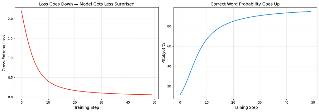
The left chart shows loss dropping, the model gets less surprised by the right answer over time. The right chart shows P(tokyo) rising, the model becomes more confident about the correct prediction. These are real numbers from the training loop above, not simulated curves.
Part 2: Why ChatGPT’s First Word Is the Slowest: KV Caching
The Problem You Must Have Already Noticed
After you type a message in ChatGPT and hit enter, there is a pause. Then the first word appears. Then the rest of the words stream out quickly, one after another.
Why the pause? And why is the rest fast?
The answer is KV caching, a speed trick that every LLM uses.
Why Generating Text Is Slow Without Caching
Remember from the Decoder overview: generating text means predicting one word at a time. Each new word requires running attention over the entire sequence, the new word needs to attend to every word that came before it.
Without caching, the model recalculates the Key (K) and Value (V) vectors for every previous word, every single time it generates a new word. But those K and V vectors for previous words have not changed, the word “The” at position 1 produces the exact same K and V whether you are generating word 5 or word 500. Recalculating them is wasted work.
# How much wasted work happens without caching?

def work_without_cache(num_tokens):
    """Each step recomputes K, V for ALL tokens"""
    total = 0
    for step in range(1, num_tokens + 1):
        total += step  # step N processes N tokens
    return total

def work_with_cache(num_tokens):
    """First step processes all. Each following step processes only 1 new token."""
    return num_tokens + (num_tokens - 1)  # first pass + 1 per remaining token

for length in [10, 100, 500, 2000]:
    without = work_without_cache(length)
    with_c = work_with_cache(length)
    savings = (1 - with_c / without) * 100
    print(f"  {length:>5} tokens: without cache = {without:>10,} ops, "
          f"with cache = {with_c:>6,} ops, "
          f"savings = {savings:.0f}%")
10 tokens: without cache =         55 ops, with cache =     19 ops, savings = 65%
    100 tokens: without cache =      5,050 ops, with cache =    199 ops, savings = 96%
    500 tokens: without cache =    125,250 ops, with cache =    999 ops, savings = 99%
   2000 tokens: without cache =  2,001,000 ops, with cache =  3,999 ops, savings = 100%
For a 2000-token response, caching eliminates over 99% of redundant computation. That is the difference between a response taking seconds versus minutes.
How KV Caching Works
The idea is dead simple: store the K and V vectors from previous tokens. When generating a new token, only compute Q, K, V for the new token. For attention, use the new Q with all the stored K and V vectors.
from scipy.special import softmax

d_k = 8
np.random.seed(42)

all_embeddings = np.random.randn(10, d_k)
W_Q = np.random.randn(d_k, d_k) * 0.3
W_K = np.random.randn(d_k, d_k) * 0.3
W_V = np.random.randn(d_k, d_k) * 0.3

# --- WITHOUT CACHE: generating token 5 ---
seq = all_embeddings[:5]
Q_all = seq @ W_Q    # compute Q for ALL 5 tokens
K_all = seq @ W_K    # compute K for ALL 5 tokens
V_all = seq @ W_V    # compute V for ALL 5 tokens

scores = Q_all[-1:] @ K_all.T / np.sqrt(d_k)
weights = softmax(scores, axis=-1)
output_no_cache = weights @ V_all

print("WITHOUT Cache — generating token 5:\n")
print(f"  Q shape: {Q_all.shape} — computed for all 5 tokens")
print(f"  K shape: {K_all.shape} — computed for all 5 tokens")
print(f"  V shape: {V_all.shape} — computed for all 5 tokens")
print(f"  K,V computations: {K_all.shape[0]}")
print(f"  Output: {output_no_cache.round(3)}")

# --- WITH CACHE: generating token 5 ---
# Tokens 1-4 were already processed in earlier steps — K,V are cached
cache_K = all_embeddings[:4] @ W_K
cache_V = all_embeddings[:4] @ W_V

# Only compute Q, K, V for the NEW token (token 5)
new_token = all_embeddings[4:5]
Q_new = new_token @ W_Q
K_new = new_token @ W_K
V_new = new_token @ W_V

# Append new K, V to the cache
K_full = np.vstack([cache_K, K_new])
V_full = np.vstack([cache_V, V_new])

scores = Q_new @ K_full.T / np.sqrt(d_k)
weights = softmax(scores, axis=-1)
output_with_cache = weights @ V_full

print(f"\nWITH Cache — generating token 5:\n")
print(f"  From cache — K: {cache_K.shape}, V: {cache_V.shape} (4 tokens, already stored)")
print(f"  New token  — Q: {Q_new.shape}, K: {K_new.shape}, V: {V_new.shape} (1 token, computed now)")
print(f"  After append — K: {K_full.shape}, V: {V_full.shape} (cache + new)")
print(f"  K,V computations: {K_new.shape[0]} (saved {cache_K.shape[0]})")
print(f"  Output: {output_with_cache.round(3)}")

# --- PROOF ---
print(f"\n  Outputs match: {np.allclose(output_no_cache, output_with_cache)}")
print(f"  Identical result. Without cache: {K_all.shape[0]} K,V computations. With cache: {K_new.shape[0]}.")
WITHOUT Cache — generating token 5:

  Q shape: (5, 8) — computed for all 5 tokens
  K shape: (5, 8) — computed for all 5 tokens
  V shape: (5, 8) — computed for all 5 tokens
  K,V computations: 5
  Output: [[-0.643 -0.472  0.409 -0.555 -0.63  -0.255  0.962  0.02 ]]

WITH Cache — generating token 5:

  From cache — K: (4, 8), V: (4, 8) (4 tokens, already stored)
  New token  — Q: (1, 8), K: (1, 8), V: (1, 8) (1 token, computed now)
  After append — K: (5, 8), V: (5, 8) (cache + new)
  K,V computations: 1 (saved 4)
  Output: [[-0.643 -0.472  0.409 -0.555 -0.63  -0.255  0.962  0.02 ]]

  Outputs match: True
  Identical result. Without cache: 5 K,V computations. With cache: 1.
The outputs are identical. The attention result is exactly the same whether you recompute everything or use the cache. KV caching changes nothing about the answer, it only eliminates redundant work.
Visualizing the Savings
words = ["The", "capital", "of", "Japan", "is", "Tokyo", "!"]

without_cache = list(range(1, len(words) + 1))
with_cache = [1] + [1] * (len(words) - 1)  # first step full, rest = 1

fig, ax = plt.subplots(figsize=(12, 5))
x = np.arange(len(words))
width = 0.35

bars1 = ax.bar(x - width/2, without_cache, width, label="Without KV Cache",
               color="#e74c3c", alpha=0.8)
bars2 = ax.bar(x + width/2, with_cache, width, label="With KV Cache",
               color="#3498db", alpha=0.8)

ax.set_xlabel("Generation Step", fontsize=12)
ax.set_ylabel("K,V Computations", fontsize=12)
ax.set_title("KV Caching — Computation Per Step", fontsize=14)
ax.set_xticks(x)
ax.set_xticklabels([f'"{w}"' for w in words], fontsize=10)
ax.legend(fontsize=11)
ax.grid(True, alpha=0.3, axis='y')

for bar in bars1:
    ax.text(bar.get_x() + bar.get_width()/2., bar.get_height() + 0.1,
            f'{int(bar.get_height())}', ha='center', va='bottom', fontsize=9)
for bar in bars2:
    ax.text(bar.get_x() + bar.get_width()/2., bar.get_height() + 0.1,
            f'{int(bar.get_height())}', ha='center', va='bottom', fontsize=9)

plt.tight_layout()
plt.show()
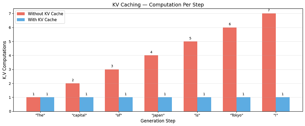
Red bars grow with each step, without caching, more and more work piles up. Blue bars stay flat at 1, with caching, every step after the first does the same small amount of work. Same output, fraction of the cost.
Why the First Word Is Slow, and the Rest Are Fast
Now the answer is clear:
The first word (slow): The model has to process the entire prompt, every word, through every layer. This is called the prefill phase. It is the first time seeing these tokens, so there is nothing to cache yet. All K and V vectors are computed fresh and stored.
Every word after that (fast): The K and V vectors for previous words are already in the cache. The model only computes Q, K, V for the one new token and looks up everything else. This is the decode phase.
The pause you see before ChatGPT starts responding? That is the prefill. The fast streaming after? That is decode with KV caching.
The Trade-Off: Speed Costs Memory
KV caching speeds up generation dramatically, but it is not free. Every cached K and V vector takes up GPU memory. For a large model with many layers and a long conversation, that memory adds up.
# How much memory does the KV cache use?

d_model = 4096       # typical for a large model
n_layers = 32        # Transformer layers
seq_len = 4096       # context window
bytes_per_value = 2  # FP16 precision

# Each layer caches K and V, each of shape (seq_len, d_model)
cache_per_sequence = 2 * n_layers * seq_len * d_model * bytes_per_value
cache_gb = cache_per_sequence / (1024 ** 3)

print("KV Cache Memory:\n")
print(f"  Model: {d_model}-dim, {n_layers} layers")
print(f"  Precision: FP16 (2 bytes per number)\n")

for ctx_len in [1024, 4096, 16384, 128000]:
    cache = 2 * n_layers * ctx_len * d_model * bytes_per_value / (1024**3)
    print(f"  Context {ctx_len:>7,} tokens → {cache:.2f} GB per conversation")

print(f"\n  This is per conversation. Serving 100 users simultaneously")
print(f"  at 4096 context = {cache_gb * 100:.0f} GB just for the cache.")
print(f"  This is why longer context windows cost more to serve.")
KV Cache Memory:

  Model: 4096-dim, 32 layers
  Precision: FP16 (2 bytes per number)

  Context   1,024 tokens → 0.50 GB per conversation
  Context   4,096 tokens → 2.00 GB per conversation
  Context  16,384 tokens → 8.00 GB per conversation
  Context 128,000 tokens → 62.50 GB per conversation

  This is per conversation. Serving 100 users simultaneously
  at 4096 context = 200 GB just for the cache.
  This is why longer context windows cost more to serve.
Doubling the context window doubles the cache memory. This is the real reason why long-context models are expensive to run, it is not just the computation, it is the memory each conversation occupies on the GPU.
The Key Takeaways
Training a Decoder is conceptually simple: predict the next word, measure how wrong you were with cross-entropy loss, nudge the weights to be less wrong, repeat. Teacher forcing makes this efficient by processing all positions in parallel, the masked attention ensures no position can see the future, even though the entire sequence is present.
KV caching is what makes autoregressive generation usable in practice. Without it, each new word would require reprocessing the entire sequence from scratch. With it, only the new token is computed, everything else is looked up from the cache. The cost is memory, every conversation holds its own cache, and longer conversations use more.
The pause before ChatGPT’s first word? That is prefill, processing the entire prompt and building the cache. The fast streaming after? That is decode, one new token per step, with everything else cached. Now you know why.
That Pause Before ChatGPT Responds? Here’s What’s Actually Happening was originally published in Level Up Coding on Medium, where people are continuing the conversation by highlighting and responding to this story.