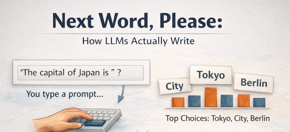
You type “The capital of Japan is” and GPT responds “Tokyo!” But how? It does not search a database. It does not look up the answer. It predicts the next word, one token at a time. This article explains how.
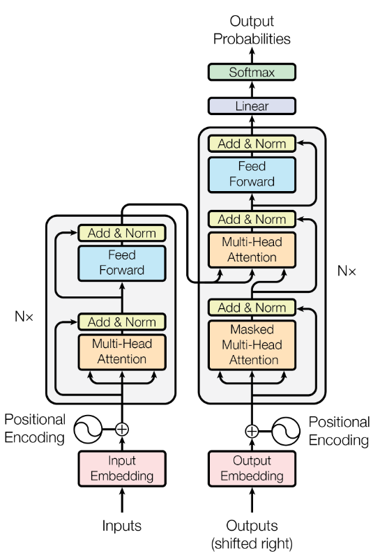
The previous articles in this series covered how Transformers understand language, embeddings turn words into numbers, positional encoding adds word order, attention figures out which words matter, and Layer Norm and feed-forward networks refine the representation. All of that is the input side of the story.
This article is about the output side. How does a Transformer actually generate text? How does it go from understanding “The capital of Japan is” to producing “Tokyo”?
The answer is the Decoder.
Encoder vs. Decoder: The Big Picture
Before diving into how the Decoder works, it helps to understand where it fits.
A Transformer can be built in three ways:
Encoder-only (like BERT). Reads the entire input at once. Great for understanding, classification, sentiment analysis, extracting information. It sees all words simultaneously. But it does not generate new text.
Decoder-only (like GPT). Reads input left to right (as we humans do) and generates output one word at a time. This is what powers ChatGPT, Claude, LLaMA, and most modern language models. It only looks backward, each word can only see the words that came before it.
Encoder-Decoder (like the original Transformer, T5). The encoder reads the full input (like a sentence in French), then the decoder generates the output one word at a time (the English translation). Used for translation, summarization, and tasks where you need to process one thing and produce another.
The Decoder-only architecture is what dominates today. When people say “LLM,” they almost always mean a Decoder. This article focuses on how it works.
The Core Idea: Next-Token Prediction
The entire job of a Decoder can be described in one sentence: given all the words so far, predict the next one.
That’s it. Every response GPT has ever generated, every essay, every code snippet, every conversation, was produced by doing this one thing over and over.
Here is how “The capital of Japan is Tokyo!” gets generated:
Step 1: Input "The"               → Model predicts: "capital"
Step 2: Input "The capital"        → Model predicts: "of"
Step 3: Input "The capital of"     → Model predicts: "Japan"
Step 4: Input "The capital of Japan" → Model predicts: "is"
Step 5: Input "The capital of Japan is" → Model predicts: "Tokyo"
Step 6: Input "The capital of Japan is Tokyo" → Model predicts: "!" (or stop)
Each step feeds the full sequence so far into the model, and the model predicts one more word. Then that word is added to the sequence, and the process repeats. This is called autoregressive generation, the model’s own output becomes part of its next input.
import numpy as np
from scipy.special import softmax

def masked_attention(Q, K, V):
    d_k = Q.shape[-1]
    seq_len = Q.shape[0]
    scores = Q @ K.T / np.sqrt(d_k)
    mask = np.triu(np.ones((seq_len, seq_len)), k=1)
    scores = scores - mask * 1e9
    weights = softmax(scores, axis=-1)
    return weights @ V, weights

# Setup
np.random.seed(42)
vocab = ["the", "capital", "of", "japan", "is", "tokyo", "city", "berlin", "!", "<stop>"]
vocab_size = len(vocab)
d_model = 16

embedding_table = np.random.randn(vocab_size, d_model) * 0.5
W_Q = np.random.randn(d_model, d_model) * 0.3
W_K = np.random.randn(d_model, d_model) * 0.3
W_V = np.random.randn(d_model, d_model) * 0.3
W_output = np.random.randn(d_model, vocab_size) * 0.3

def generate_next(sequence_ids):
    embeddings = embedding_table[sequence_ids]
    Q = embeddings @ W_Q
    K = embeddings @ W_K
    V = embeddings @ W_V
    attended, _ = masked_attention(Q, K, V)
    last_token = attended[-1]
    logits = last_token @ W_output
    return softmax(logits)

prompt = ["the", "capital", "of"]
sequence = [vocab.index(w) for w in prompt]

print("Autoregressive Generation:\n")
print(f"  Prompt: '{' '.join(prompt)}'\n")

for step in range(2):
    probs = generate_next(np.array(sequence))
    next_id = np.argmax(probs)
    next_word = vocab[next_id]
    context = " ".join([vocab[i] for i in sequence])

    sorted_indices = np.argsort(probs)[::-1][:3]
    top_3 = [(vocab[i], probs[i]) for i in sorted_indices]

    print(f"  Step {step + 1}: '{context}'")
    print(f"    Top predictions: {top_3[0][0]} ({top_3[0][1]:.1%}), {top_3[1][0]} ({top_3[1][1]:.1%}), {top_3[2][0]} ({top_3[2][1]:.1%})")
    print(f"    Picked: '{next_word}'\n")

    sequence.append(next_id)

print(f"  Generated so far: '{' '.join([vocab[i] for i in sequence])}'")
Autoregressive Generation:

  Prompt: 'the capital of'

  Step 1: 'the capital of'
    Top predictions: japan (21.9%), city (13.1%), berlin (13.0%)
    Picked: 'japan'

  Step 2: 'the capital of japan'
    Top predictions: tokyo (15.6%), japan (12.5%), city (12.0%)
    Picked: 'tokyo'

  Generated so far: 'the capital of japan tokyo'
The model predicts “japan” then “tokyo”, with untrained random weights, this is coincidence, not understanding. But the mechanism is exactly what a real LLM does: embed the sequence, run masked attention, score every word in the vocabulary, and pick the highest. Training on trillions of words is what turns this process into one that reliably produces the right answer.
Why One Word at a Time?
This might seem slow. Why not generate the whole sentence at once?
The answer is that each word depends on the words before it. The model cannot predict “Tokyo” without first knowing the sentence is about “capital” and “Japan.” By generating one word at a time, each prediction has full context from everything generated so far.
This is the fundamental difference from the Encoder. An Encoder sees all words simultaneously, it reads the whole sentence at once. A Decoder sees words one by one, left to right, building the output token by token. This brings us to our next topic understanding “Masked Self-Attention.”
Masked Self-Attention: No Peeking Ahead
The previous article on attention explained how every word can attend to every other word. In the Encoder, “cat” can look at “sat,” and “sat” can look at “cat.” Every word sees every other word, including words that come after it.
The Decoder cannot allow this. If the model is predicting the word at position 5, it must not see positions 6, 7, 8, and beyond, those words have not been generated yet. Letting the model see future words during training would be cheating, and the model would fail at generation time when those future words do not exist.
The solution is masked self-attention. It works exactly like regular self-attention, but with a mask that blocks all positions ahead of the current one.
import numpy as np
from scipy.special import softmax

def masked_attention(Q, K, V):
    """Self-attention with a causal mask — no looking ahead"""
    d_k = Q.shape[-1]
    seq_len = Q.shape[0]

    scores = Q @ K.T / np.sqrt(d_k)
    mask = np.triu(np.ones((seq_len, seq_len)), k=1)
    scores = scores - mask * 1e9
    weights = softmax(scores, axis=-1)
    output = weights @ V

    return output, weights

# Simulate a 5-word sequence
np.random.seed(42)
seq_len = 5
d_k = 8

Q = np.random.randn(seq_len, d_k)
K = np.random.randn(seq_len, d_k)
V = np.random.randn(seq_len, d_k)

output, weights = masked_attention(Q, K, V)

words = ["The", "capital", "of", "Japan", "is"]
print("Masked Attention Weights:\n")
print(f"{'':>12}", end="")
for w in words:
    print(f"{w:>10}", end="")
print()

for i, word in enumerate(words):
    print(f"{word:>12}", end="")
    for j in range(len(words)):
        print(f"{weights[i][j]:>10.3f}", end="")
    print()
Masked Attention Weights:

                   The   capital        of     Japan        is
         The     1.000     0.000     0.000     0.000     0.000
     capital     0.889     0.111     0.000     0.000     0.000
          of     0.166     0.210     0.624     0.000     0.000
       Japan     0.384     0.157     0.101     0.358     0.000
          is     0.390     0.197     0.266     0.110     0.036
Look at the pattern: “The” can only attend to itself. “Capital” can attend to “The” and itself. “Of” can attend to “The,” “capital,” and itself. Each word can only see words at or before its own position. The future is invisible.
Visualizing the Mask
import matplotlib.pyplot as plt
from scipy.special import softmax

fig, axes = plt.subplots(1, 2, figsize=(16, 6))

# Encoder attention (no mask — everyone sees everyone)
encoder_weights = softmax(np.random.randn(5, 5), axis=-1)

ax1 = axes[0]
ax1.imshow(encoder_weights, cmap="Blues", vmin=0, vmax=0.6)
ax1.set_xticks(range(5))
ax1.set_xticklabels(words, fontsize=11)
ax1.set_yticks(range(5))
ax1.set_yticklabels(words, fontsize=11)
ax1.set_title("Encoder: Full Attention\n(every word sees every word)", fontsize=13)
ax1.set_xlabel("Attending To", fontsize=11)
ax1.set_ylabel("Current Word", fontsize=11)
for i in range(5):
    for j in range(5):
        ax1.text(j, i, f"{encoder_weights[i][j]:.2f}", ha="center", va="center",
                fontsize=9, color="white" if encoder_weights[i][j] > 0.3 else "black")

# Decoder attention (masked — only see past)
ax2 = axes[1]
ax2.imshow(weights, cmap="Blues", vmin=0, vmax=0.6)
ax2.set_xticks(range(5))
ax2.set_xticklabels(words, fontsize=11)
ax2.set_yticks(range(5))
ax2.set_yticklabels(words, fontsize=11)
ax2.set_title("Decoder: Masked Attention\n(each word only sees past + itself)", fontsize=13)
ax2.set_xlabel("Attending To", fontsize=11)
ax2.set_ylabel("Current Word", fontsize=11)
for i in range(5):
    for j in range(5):
        ax2.text(j, i, f"{weights[i][j]:.2f}", ha="center", va="center",
                fontsize=9, color="white" if weights[i][j] > 0.3 else "black")

plt.tight_layout()
plt.savefig("encoder_vs_decoder_attention.png", dpi=150, bbox_inches="tight")
plt.show()
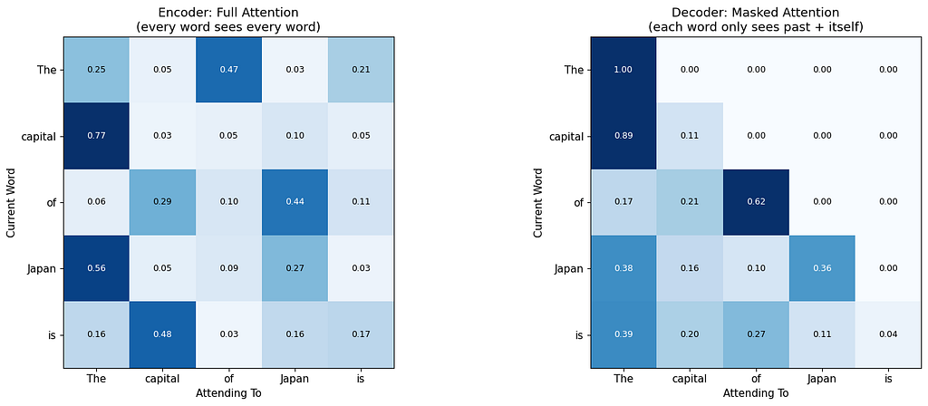
The Encoder heatmap is full, every cell has a non-zero value. The Decoder heatmap has a triangle, the upper right is all zeroes. That triangle is the mask, and it is the single biggest difference between an Encoder and a Decoder.
From Attention to Prediction: The Output Layer
After the masked attention, layer norm, and feed-forward network process the input (all the same components from previous articles), the Decoder needs to make an actual prediction. It needs to say: “The next word is Tokyo.”
This happens in two steps:
Step 1: Take the last token’s embedding. After passing through all the Transformer layers, every word in the input has a rich, contextualized embedding. But the model only needs the last one, because the last position is where the “next word” prediction lives.
Step 2: Project to vocabulary. The last token’s embedding (a vector of, say, 768 numbers) is multiplied by a matrix that converts it into a score for every word in the vocabulary. If the vocabulary has 50,000 words, the result is 50,000 scores, one for each possible next word.
# Simulating the output layer
np.random.seed(42)
d_model = 8
vocab_size = 10

vocab = ["the", "capital", "of", "japan", "is", "tokyo", "london", "berlin", "was", "country"]

last_token_embedding = np.array([0.8, -0.3, 1.2, 0.5, -0.7, 0.9, -0.1, 0.4])

W_output = np.random.randn(d_model, vocab_size) * 0.5

logits = last_token_embedding @ W_output

print("Raw scores (logits) for each word in vocabulary:\n")
for word, score in sorted(zip(vocab, logits), key=lambda x: -x[1]):
    bar = "█" * int(max(0, (score + 2) * 5))
    print(f"  {word:>10}: {score:>6.2f}  {bar}")
Raw scores (logits) for each word in vocabulary:

     country:   0.99  ██████████████
         the:   0.98  ██████████████
       japan:   0.53  ████████████
       tokyo:   0.52  ████████████
          is:   0.46  ████████████
     capital:   0.43  ████████████
          of:   0.04  ██████████
      london:  -0.05  █████████
      berlin:  -0.62  ██████
         was:  -0.71  ██████
These raw scores are called logits. Higher logits mean the model thinks that word is more likely to come next. But they are not probabilities yet, they are just numbers.
Turning Scores into Probabilities: Softmax
To get actual probabilities, the logits are passed through softmax (the same function used in attention from Encoder side). This converts the raw scores into a probability distribution where all values are between 0 and 1 and sum to 1.
from scipy.special import softmax

probabilities = softmax(logits)

print("Probabilities after softmax:\n")
for word, prob in sorted(zip(vocab, probabilities), key=lambda x: -x[1]):
    bar = "█" * int(prob * 50)
    print(f"  {word:>10}: {prob:>6.1%}  {bar}")

print(f"\n  Total: {probabilities.sum():.1%}")
Probabilities after softmax:

     country:  18.1%  █████████
         the:  17.9%  ████████
       japan:  11.4%  █████
       tokyo:  11.3%  █████
          is:  10.7%  █████
     capital:  10.3%  █████
          of:   7.0%  ███
      london:   6.4%  ███
      berlin:   3.6%  █
         was:   3.3%  █

  Total: 100.0%
Now the model has a probability distribution over the entire vocabulary. The word with the highest probability is the model’s best guess for what comes next.
How the Model Picks a Word: Sampling Strategies
The model now has a probability for every word in the vocabulary. But how does it actually choose which word to output? There are several strategies, and which one you use dramatically affects how the output reads.
Greedy Decoding: Always Pick the Most Likely
The simplest approach: always pick the word with the highest probability.
# Greedy decoding
best_word_idx = np.argmax(probabilities)
print(f"Greedy decoding picks: '{vocab[best_word_idx]}' (probability: {probabilities[best_word_idx]:.1%})")
Greedy decoding picks: 'country' (probability: 18.1%)
This is predictable and deterministic, the same input always produces the same output. Good for factual answers. Bad for creative writing, because it always takes the safest, most obvious path.
Temperature: Controlling Randomness
Temperature is a single number that controls how “creative” or “conservative” the model is. It is applied to the logits before softmax.
Low temperature (0.2): Makes the distribution sharper, the top word gets even more probability, and unlikely words get almost none. The model is very confident and predictable.
High temperature (1.5): Makes the distribution flatter, probabilities spread out more evenly. The model takes more risks and produces more surprising (sometimes nonsensical) output.
Temperature = 1.0: The default, probabilities are used as the model learned them.
from scipy.special import softmax

def apply_temperature(logits, temperature):
    return softmax(logits / temperature)

temperatures = [0.2, 0.7, 1.0, 1.5]

print("How temperature changes the probability distribution:\n")
for temp in temperatures:
    probs = apply_temperature(logits, temp)

    print(f"  Temperature {temp}:")
    sorted_indices = np.argsort(probs)[::-1]
    for idx in sorted_indices[:3]:
        bar = "█" * int(probs[idx] * 40)
        print(f"    {vocab[idx]:>10}: {probs[idx]:>6.1%}  {bar}")
    print()
How temperature changes the probability distribution:

  Temperature 0.2:
       country:  44.0%  █████████████████
           the:  41.2%  ████████████████
         japan:   4.3%  █

  Temperature 0.7:
       country:  21.8%  ████████
           the:  21.4%  ████████
         japan:  11.2%  ████

  Temperature 1.0:
       country:  18.1%  ███████
           the:  17.9%  ███████
         japan:  11.4%  ████

  Temperature 1.5:
       country:  15.3%  ██████
           the:  15.2%  ██████
         japan:  11.2%  ████
Lower temperature, safer answers. Higher temperature, wilder answers. That single number controls the balance between predictable and creative, across every LLM.
Top-k Sampling: Only Consider the Best Options
Instead of choosing from the entire vocabulary, top-k sampling first narrows down to the k most likely words, then samples from those.
from scipy.special import softmax

def apply_temperature(logits, temperature):
    return softmax(logits / temperature)

def top_k_sampling(logits, k, temperature=1.0):
    probs = apply_temperature(logits, temperature)

    top_k_indices = np.argsort(probs)[::-1][:k]
    top_k_probs = probs[top_k_indices]
    top_k_probs = top_k_probs / top_k_probs.sum()

    chosen_idx = np.random.choice(top_k_indices, p=top_k_probs)

    return vocab[chosen_idx], top_k_probs, [vocab[i] for i in top_k_indices]

np.random.seed(42)
print("Top-k sampling (k=3):\n")
for trial in range(5):
    word, probs, candidates = top_k_sampling(logits, k=3)
    print(f"  Trial {trial + 1}: Candidates {candidates} → picked '{word}'")
Top-k sampling (k=3):

  Trial 1: Candidates ['country', 'the', 'japan'] → picked 'country'
  Trial 2: Candidates ['country', 'the', 'japan'] → picked 'japan'
  Trial 3: Candidates ['country', 'the', 'japan'] → picked 'the'
  Trial 4: Candidates ['country', 'the', 'japan'] → picked 'the'
  Trial 5: Candidates ['country', 'the', 'japan'] → picked 'country'
Top-k prevents the model from ever choosing a very unlikely word. If k=3, the model can only pick from its top 3 choices. This avoids nonsensical outputs while still allowing some variety.
Top-p (Nucleus) Sampling: Dynamic Cutoff
Top-p is similar to top-k, but instead of a fixed number of candidates, it includes words until their combined probability reaches a threshold p.
def top_p_sampling(logits, p, temperature=1.0):
    """Include words until cumulative probability reaches p"""
    probs = apply_temperature(logits, temperature)

    # Sort by probability (highest first)
    sorted_indices = np.argsort(probs)[::-1]
    sorted_probs = probs[sorted_indices]

    # Find cutoff where cumulative probability reaches p
    cumulative = np.cumsum(sorted_probs)
    cutoff = np.searchsorted(cumulative, p) + 1

    # Keep only words within the nucleus
    nucleus_indices = sorted_indices[:cutoff]
    nucleus_probs = probs[nucleus_indices]
    nucleus_probs = nucleus_probs / nucleus_probs.sum()

    chosen_idx = np.random.choice(nucleus_indices, p=nucleus_probs)

    return vocab[chosen_idx], cutoff, [vocab[i] for i in nucleus_indices]

np.random.seed(42)
print("Top-p sampling (p=0.9):\n")
for trial in range(5):
    word, n_candidates, candidates = top_p_sampling(logits, p=0.9)
    print(f"  Trial {trial + 1}: Nucleus = {candidates} ({n_candidates} words) → picked '{word}'")
Top-p sampling (p=0.9):

  Trial 1: Nucleus = ['country', 'the', 'japan', 'tokyo', 'is', 'capital', 'of', 'london'] (8 words) → picked 'the'
  Trial 2: Nucleus = ['country', 'the', 'japan', 'tokyo', 'is', 'capital', 'of', 'london'] (8 words) → picked 'london'
  Trial 3: Nucleus = ['country', 'the', 'japan', 'tokyo', 'is', 'capital', 'of', 'london'] (8 words) → picked 'is'
  Trial 4: Nucleus = ['country', 'the', 'japan', 'tokyo', 'is', 'capital', 'of', 'london'] (8 words) → picked 'tokyo'
  Trial 5: Nucleus = ['country', 'the', 'japan', 'tokyo', 'is', 'capital', 'of', 'london'] (8 words) → picked 'country'
The advantage of top-p over top-k: it adapts. When the model is very confident (one word has 95% probability), the nucleus might contain just 1–2 words. When the model is uncertain (several words at 15–20% each), the nucleus expands to include more options. The cutoff is dynamic, not fixed.
Why the Decoder Architecture Dominates
Almost every major LLM today, GPT, Claude, LLaMA, Gemini, Mistral, uses a Decoder-only architecture. Why?
Simplicity. One architecture handles both understanding and generation. You do not need a separate encoder, the decoder reads the prompt and generates the response in one pass.
Scaling. Decoder-only models scale predictably. Double the parameters, double the layers, and performance improves. This made the “just make it bigger” strategy viable, leading to the massive models we see today.
Flexibility. The same model can answer questions, write code, translate languages, summarize documents, and have conversations. It is all next-token prediction, just with different prompts.
Training is straightforward. Take a massive pile of text. For every position in every sentence, train the model to predict the next word. No labels needed. No task-specific datasets. Just raw text and next-token prediction. This is why these models can be trained on trillions of words scraped from the internet.
The Decoder’s Limitations
The Decoder is powerful, but it has real constraints:
It can only look backward. Unlike an Encoder, which sees the entire input at once, the Decoder processes left to right. It cannot revise earlier words based on what comes later. Once “Tokyo” is generated, it stays, even if later context suggests “London” would have been better.
It is autoregressive, and therefore slow. Each word requires a full pass through the model. Generating a 500-word response means 500 forward passes. This is why LLMs have noticeable latency, and why optimizations like KV (key-value) caching (storing intermediate attention results) are critical for speed.
It can hallucinate. Since the model picks the most probable next token based on patterns it saw in training, it can produce confident-sounding text that is factually wrong. It is not retrieving knowledge, it is predicting plausible continuations. Those are not the same thing.
Long outputs can drift. As the generated sequence gets longer, earlier context may get diluted. The model might start a paragraph about Japan and slowly drift to talking about Italy, because token-by-token prediction has no global plan for the entire output.
The Decoder is fundamentally a next-token prediction machine. It reads everything generated so far, produces a probability distribution over the entire vocabulary, picks one word, adds it to the sequence, and repeats.
Masked self-attention is what makes this possible, it ensures that during both training and generation, each word can only see the words that came before it. No peeking ahead.
The output layer converts the final embedding into vocabulary scores, and sampling strategies (greedy, temperature, top-k, top-p) control how the model chooses from those scores.
Every conversation with ChatGPT, every code snippet from Copilot, every translation from a modern model, it all comes down to one operation repeated thousands of times: read what came before, predict what comes next.
Next Word, Please: How LLMs Actually Write was originally published in Level Up Coding on Medium, where people are continuing the conversation by highlighting and responding to this story.