Market Regimes in Indian Stocks: Detecting Market Regimes with a Hidden Markov Model — How a Hidden…

Market Regimes in Indian Stocks: Detecting Market Regimes with a Hidden Markov Model — How a Hidden Markov Model Reveals Market Regimes

Is the Market About to Crash? I Built an AI to Find Out.

Can machine learning detect market regimes in financial markets?

Most investors believe that financial markets move through different market regimes.

Some periods are dominated by strong upward trends.
Others are marked by crashes, uncertainty, or sideways trading.

Common examples include:

Bull markets
Market crashes
Sideways consolidation
High volatility phases

But here is the key question:

Can machine learning automatically detect market regimes from data?

To explore this idea, I built a small experiment using Python and a Hidden Markov Model to analyze Indian stock market data.

What Are Market Regimes?

Q: What exactly is a market regime?

A market regime refers to a period where financial markets exhibit relatively consistent behavior.

For example:

Instead of assuming markets behave the same way over time, regime theory suggests that markets transition between different states.

Q: Why do market regimes exist?

Market regimes emerge because the economic environment constantly changes.

Some major drivers include:

economic growth cycles
interest rate changes
geopolitical events
liquidity conditions
investor sentiment

For example:

• During economic expansion → growth stocks often dominate
• During crises → defensive sectors tend to outperform
• During uncertainty → volatility increases significantly

These shifts create patterns in financial data that machine learning models can detect.

Step 1 — Collecting Market Data

To detect market regimes, we first need market data.

In Python, one of the easiest ways to obtain financial data is the yfinance library, which allows direct downloads from Yahoo Finance.

Below is a simple example using the NIFTY 50 index.

import yfinance as yf
import pandas as pd

tickers = ["^NSEI"]

data = yf.download(tickers, start="2015-01-01", end="2025-01-01")

returns = data['Close'].pct_change().dropna()

This gives us daily market returns over a 10-year period.

These returns form the foundation for identifying market regimes.

How Can We Observe Market Regimes Using Data Analytics?

Financial datasets do not explicitly label market regimes.

There is no column like:

Market_State = "Crash"

Instead, regimes must be inferred from patterns in financial data.

Analysts typically examine indicators such as:

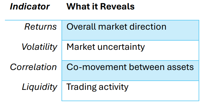
Using these indicators, we can begin to observe behavioral patterns in markets.

For example:

High volatility + negative returns → crisis regime
Low volatility + positive returns → expansion regime
Low volatility + flat returns → sideways regime

These signals can be extracted using statistical techniques such as:

rolling statistics
clustering methods
probabilistic models

Visualizing Market Volatility

Before applying machine learning models, it helps to visualize how volatility changes over time.

Volatility often increases sharply during periods of market stress.

import matplotlib.pyplot as plt
import yfinance as yf

data = yf.download("^NSEI", start="2015-01-01", end="2025-01-01")

prices = data["Close"]
returns = prices.pct_change()

volatility = returns.rolling(20).std()

plt.figure(figsize=(12,5))
plt.plot(volatility, label="20-Day Rolling Volatility")

plt.title("Market Volatility in NIFTY 50 (2015–2025)")
plt.xlabel("Date")
plt.ylabel("Volatility")
plt.legend()

plt.show()

When you plot this chart, you will notice clusters of volatility.

For example, volatility spikes significantly around 2020, reflecting the global market disruption caused by COVID-19.

These clusters are strong indicators that markets move through different market regimes.

Step 2 — Feature Engineering

Next, we create features that help a machine learning model detect regime changes.

Three useful features include:

Market growth
Interest rate changes
Market volatility

In this simplified example, we estimate growth and volatility using rolling statistics.

returns["growth"] = returns.rolling(20).mean()
returns["vol"] = returns.rolling(20).std()

import yfinance as yf
import pandas as pd
import matplotlib.pyplot as plt

# Step 1: Download NIFTY data
data = yf.download(
    "^NSEI",
    start="2015-01-01",
    end="2025-01-01",
    auto_adjust=True
)

# Step 2: Extract closing prices
prices = data["Close"]

# Step 3: Compute returns
returns = prices.pct_change().dropna()

# Convert to DataFrame safely
returns = pd.DataFrame(returns)
returns.columns = ["returns"]

# Step 4: Feature Engineering
returns["growth"] = returns["returns"].rolling(20).mean()
returns["vol"] = returns["returns"].rolling(20).std()

# Drop NaN rows from rolling window
returns = returns.dropna()

# Step 5: View dataset
print(returns.head())

# Step 6: Visualization
plt.figure(figsize=(12,5))

plt.plot(returns.index, returns["growth"], label="20-Day Growth")
plt.plot(returns.index, returns["vol"], label="20-Day Volatility")

plt.title("NIFTY Market Growth vs Volatility")
plt.xlabel("Date")
plt.ylabel("Value")
plt.legend()

plt.show()

These features help capture how market conditions evolve over time.

Which Machine Learning Models Can Detect Market Regimes?

Several machine learning models can be used for regime detection.

Some common approaches include:

Among these, the Hidden Markov Model is one of the most widely used models in quantitative finance.

Why Hidden Markov Models Work Well

A Hidden Markov Model is particularly suited for regime detection because it assumes:

Markets exist in hidden states
These states evolve over time
The probability of switching between states can be modeled

For example, markets may transition like this:

Bull Market → Bull Market → Bull Market → Volatility Spike → Crash

The Hidden Markov Model estimates the probability of moving between these states.

Another advantage is that the model captures time dependence, meaning today’s state depends on yesterday’s state.

This characteristic aligns closely with how financial markets behave.

Models That Are Not Ideal for Regime Detection

Not all machine learning models work well for detecting market regimes.

Some models assume static relationships rather than dynamic transitions.

Examples include:

These models focus on predicting outcomes, whereas regime detection requires identifying structural market states.

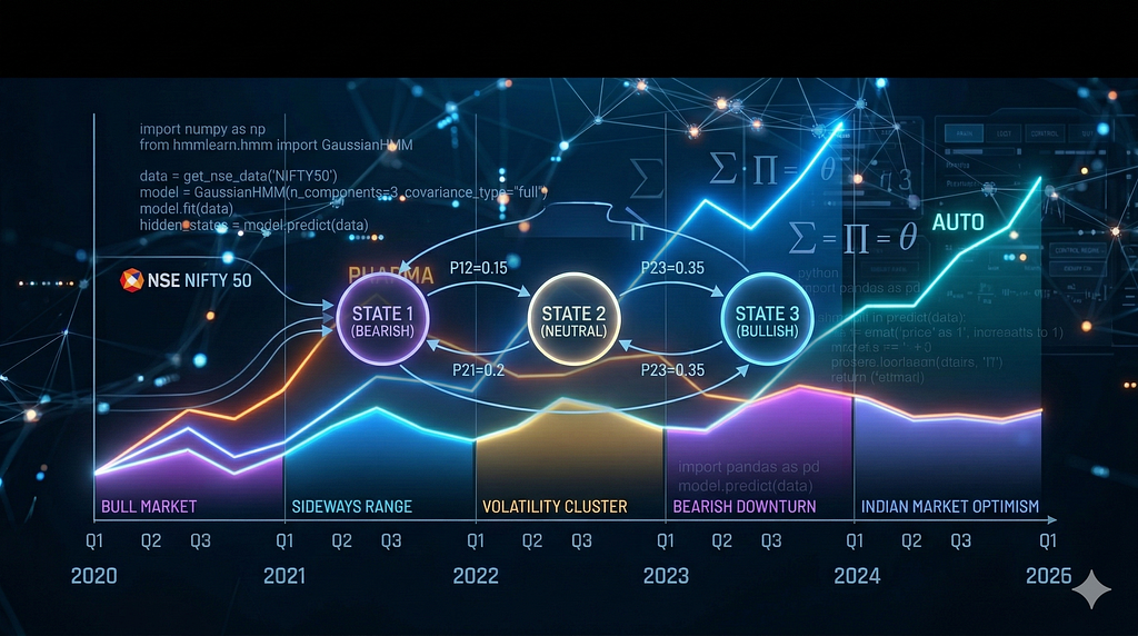
Step 3 — Detecting Market Regimes with a Hidden Markov Model

Now we implement the Hidden Markov Model.

from hmmlearn.hmm import GaussianHMM 

model = GaussianHMM(n_components=3)

model.fit(returns.dropna()) 

regimes = model.predict(returns.dropna())

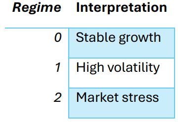
The model classifies the market into three regimes.

Typically they correspond to:

Visualizing Detected Market Regimes

import matplotlib.pyplot as plt 

plt.scatter(returns.index, returns['growth'], c=regimes) 
plt.show()

import yfinance as yf
import pandas as pd
import matplotlib.pyplot as plt
from hmmlearn.hmm import GaussianHMM

# -----------------------------
# Step 1: Download NIFTY data
# -----------------------------
data = yf.download(
    "^NSEI",
    start="2015-01-01",
    end="2025-01-01",
    auto_adjust=True
)

# -----------------------------
# Step 2: Prepare price data
# -----------------------------
prices = data["Close"]

# Compute returns
returns = prices.pct_change().dropna()

# Convert to DataFrame
returns = pd.DataFrame(returns)
returns.columns = ["returns"]

# -----------------------------
# Step 3: Feature Engineering
# -----------------------------
returns["growth"] = returns["returns"].rolling(20).mean()
returns["vol"] = returns["returns"].rolling(20).std()

returns = returns.dropna()

# -----------------------------
# Step 4: Train HMM model
# -----------------------------
features = returns[["growth", "vol"]]

model = GaussianHMM(n_components=3, covariance_type="full", n_iter=1000)

model.fit(features)

regimes = model.predict(features)

# -----------------------------
# Step 5: Scatter Visualization
# -----------------------------
plt.figure(figsize=(12,6))

plt.scatter(
    returns.index,
    returns["growth"],
    c=regimes,
    cmap="viridis",
    s=10
)

plt.title("Market Regimes Detected by Hidden Markov Model")
plt.xlabel("Date")
plt.ylabel("Market Growth")

plt.colorbar(label="Regime")

plt.show()

Each color represents a different market regime identified by the Hidden Markov Model.

Where Regime Detection Is Used in Real Finance

Market regime detection is not just theoretical.

It plays an important role in professional finance.

Hedge Fund Macro Strategies

Global macro funds analyze economic regimes such as:

expansion
recession
inflationary cycles
financial stress

These regimes influence decisions about equities, currencies, and commodities.

Volatility Trading

Options traders monitor volatility regimes to decide when to trade:

index options
volatility futures
hedging strategies

Volatility spikes often signal regime shifts.

Portfolio Risk Management

Large asset managers monitor risk-off regimes to adjust portfolio exposure.

Typical adjustments include:

reducing equity exposure
increasing cash allocations
shifting toward defensive sectors

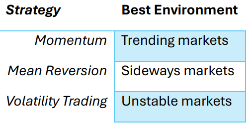
Algorithmic Trading

Quantitative trading systems often activate strategies depending on market regimes.

For example:

The Key Idea

Financial markets are not static.

They constantly move between different market regimes.

Regime detection attempts to answer one important question:

“What type of market environment are we currently in?”

But detecting regimes is only the first step.

The bigger challenge is determining whether regime detection can actually improve portfolio performance.

Can Market Regimes Improve Portfolio Strategies?

That was the next question I wanted to test.

In the next article, I build a regime-based portfolio strategy using a Hidden Markov Model and compare it with a simple diversified portfolio.

The results were surprising.

Will be continued in the next article

Market Regimes in Indian Stocks: Detecting Market Regimes with a Hidden Markov Model — How a Hidden… was originally published in DataDrivenInvestor on Medium, where people are continuing the conversation by highlighting and responding to this story.

Market Regimes in Indian Stocks: Detecting Market Regimes with a Hidden Markov Model — How a Hidden…