I Built a Regime-Based Portfolio Strategy Using Python — And Put Sector Rotation to the Test

I Built a Regime-Based Portfolio Strategy Using Python — And Put Sector Rotation to the Test

I tested whether sector rotation strategies actually work using a Hidden Markov Model and 10 years of Indian stock market data.
The results were surprising.

Finance loves clean stories.

The kind that fit neatly into textbooks:

• Auto stocks surge when the economy expands
• IT leads during innovation-driven growth
• Pharma acts as a defensive shield during crises

This narrative is the backbone of what investors call sector rotation.

It sounds elegant. Almost obvious.

But markets have a habit of humiliating obvious ideas.

So I asked a more interesting question:

Does sector rotation actually improve portfolio performance when tested against real data?

Instead of debating theory, I decided to run an experiment.

I built a regime-based portfolio strategy in Python, applied it to Indian equities, and let the data decide.

The idea was straightforward:

Detect market regimes → Allocate capital dynamically across sectors.

If sector rotation really works, the model should outperform a simple diversified portfolio.

Why Regime Detection Might Make Sector Rotation Work

Markets rarely move in straight lines. They shift between different states.

Think of them as hidden regimes:

• expansion
• volatility spikes
• systemic stress

Each environment changes the rules of the game.

Certain sectors should theoretically dominate specific regimes.

If this pattern holds, a regime-aware portfolio should have a clear edge over static allocation.

That’s the hypothesis.

Now it needed a proper test.

Step 1 — Constructing Sector Proxies

Instead of relying on sector indices, I built simple sector baskets using representative companies.

Auto sector

auto = ["MARUTI.NS","M&M.NS","EICHERMOT.NS"]

IT sector

it = ["TCS.NS","INFY.NS","HCLTECH.NS"]

Pharma sector

pharma = ["SUNPHARMA.NS","DRREDDY.NS","CIPLA.NS"]

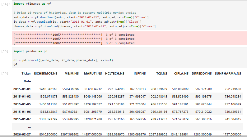
Next, I pulled historical prices using yfinance.

import yfinance as yf

# Using 10 years of historical data to capture multiple market cycles
auto_data = yf.download(auto, start="2015-01-01", auto_adjust=True)['Close']
it_data = yf.download(it, start="2015-01-01", auto_adjust=True)['Close']
pharma_data = yf.download(pharma, start="2015-01-01", auto_adjust=True)['Close']

Then I converted prices into sector-level returns.

auto_ret = auto_data.pct_change().mean(axis=1)
it_ret = it_data.pct_change().mean(axis=1)
pharma_ret = pharma_data.pct_change().mean(axis=1)

Each sector now behaves like its own synthetic index.

Clean. Simple. Comparable.

Chart 1 — Do Sectors Actually Rotate?

Before building any strategy, we need to answer a basic question:

Do these sectors actually take turns leading the market?

import matplotlib.pyplot as plt

auto_cum = (1 + auto_ret).cumprod()
it_cum = (1 + it_ret).cumprod()
pharma_cum = (1 + pharma_ret).cumprod()

plt.figure(figsize=(10,5))
plt.plot(auto_cum, label="Auto Sector")
plt.plot(it_cum, label="IT Sector")
plt.plot(pharma_cum, label="Pharma Sector")

plt.title("Sector Performance Comparison")
plt.xlabel("Date")
plt.ylabel("Cumulative Returns")
plt.legend()
plt.show()

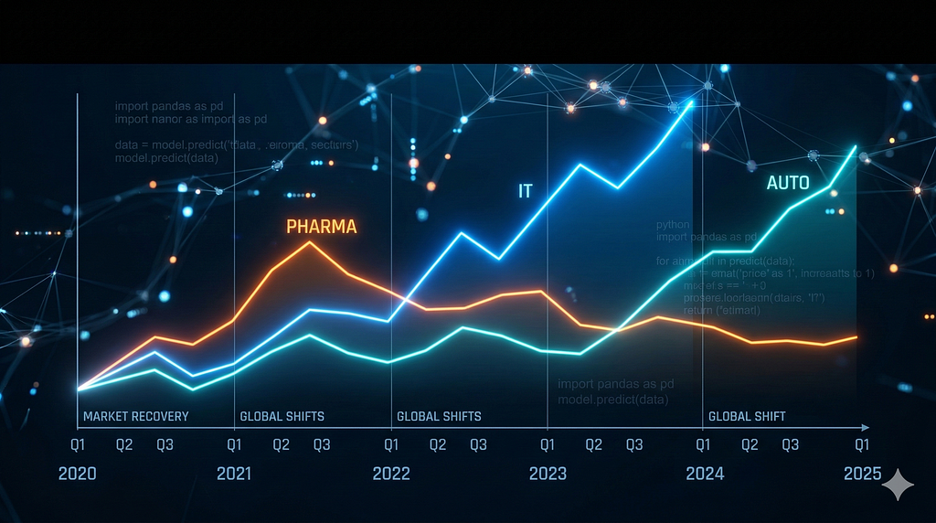
Over the 10-year period, sector leadership shifts clearly across time. Auto dominates early years, IT leads the post-COVID technology rally, and Auto regains strength in later years while Pharma behaves more defensively.

If sector rotation exists, we should see leadership shifting over time.

If not, the entire strategy collapses before it even begins.

We can observe clear leadership shifts across different periods:

• 2017–2019: Auto sector leads the market.
• 2020–2022: IT strongly outperforms, especially during the tech boom and post-COVID digital acceleration.
• 2023–2025: Auto regains leadership, while Pharma rises steadily but remains more defensive.

Step 2 — Designing the Regime-Based Allocation Model

Once a regime is detected, the portfolio adjusts its exposure.

The allocation rule is aggressive by design:

• 70% capital to the sector expected to dominate
• 15% to each of the remaining sectors

Example allocation logic:

weights = {
0: {"IT":0.7,"Auto":0.15,"Pharma":0.15},
1: {"Pharma":0.7,"IT":0.15,"Auto":0.15},
2: {"Auto":0.7,"IT":0.15,"Pharma":0.15}
}

Instead of assigning sectors manually, compute which sector has the highest average return in each regime.

Step 1 — Combine sector returns

sector_returns = pd.DataFrame({
    "Auto": auto_ret,
    "IT": it_ret,
    "Pharma": pharma_ret
})

Step 2 — Create regime labels using HMM

from hmmlearn.hmm import GaussianHMM

model = GaussianHMM(n_components=3, covariance_type="full", n_iter=1000)

model.fit(sector_returns.dropna())

regime = model.predict(sector_returns.dropna())

sector_returns = sector_returns.dropna()
sector_returns["Regime"] = regime

Step 3 — Find best sector per regime

regime_performance = sector_returns.groupby("Regime")[["Auto","IT","Pharma"]].mean()
print(regime_performance)
best_sector = regime_performance.idxmax(axis=1)
best_sector

Step 4 — Generate weights dynamically

weights = {}

for r, sector in best_sector.items():
    weights[r] = {"Auto":0.15,"IT":0.15,"Pharma":0.15}
    weights[r][sector] = 0.7

weights

Now the mapping is data-driven, not assumed.

Portfolio returns follow directly from these weights.

portfolio = []

for date, row in sector_returns.iterrows():
    
    r = int(row["Regime"])
    
    w = weights[r]
    
    p_ret = (
        w["Auto"] * row["Auto"] +
        w["IT"] * row["IT"] +
        w["Pharma"] * row["Pharma"]
    )
    
    portfolio.append(p_ret)

portfolio = pd.Series(portfolio, index=sector_returns.index)
portfolio

These weights represent one portfolio strategy, not three separate portfolios.

What you created is:

A single dynamic portfolio that changes its sector allocation depending on the detected regime.

How to interpret your result

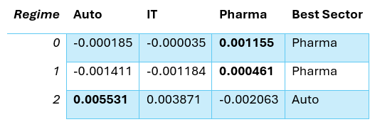
The model identified three regimes. Two regimes favoured Pharma, while one regime strongly favoured Auto.

So the model learned:

• Regime 0 → Pharma performs best
• Regime 1 → Pharma performs best
• Regime 2 → Auto performs best

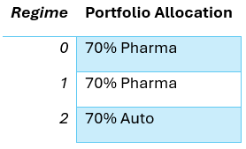
That produced these weights

{
0: {'Auto':0.15,'IT':0.15,'Pharma':0.7},
1: {'Auto':0.15,'IT':0.15,'Pharma':0.7},
2: {'Auto':0.7,'IT':0.15,'Pharma':0.15}
}

Meaning:

What happens in practice

Each day:

1. The HMM detects the current regime
2. The portfolio switches to the corresponding allocation

Example:

So it is one portfolio that changes composition over time.

Important insight from your results

Your model discovered only two effective sector regimes:

• Defensive regime → Pharma
• Growth regime → Auto

IT never became the top sector in any regime.

This is actually an interesting research result.

Interestingly, the model did not assign any regime where IT dominated. Two regimes favoured Pharma, while one favoured Auto, suggesting that defensive and cyclical dynamics were more prominent in the data than technology-driven leadership.

This becomes the engine of the regime-based portfolio strategy.

The system detects the environment.
The portfolio adapts.

In theory, this should capture sector leadership as it emerges.

Step 3 — Setting Up a Fair Benchmark

Every strategy needs a baseline.

Otherwise, you’re just admiring your own model.

The benchmark here is intentionally simple:

An equal-weight portfolio across the three sectors.

static_portfolio = (auto_ret + it_ret + pharma_ret)/3

No regime detection.
No dynamic allocation.

Just diversification.

If sector rotation truly works, the dynamic strategy should outperform this benchmark.

Chart 2 — Strategy vs Benchmark

Now the real test begins.

strategy_cum = (1 + portfolio).cumprod()
benchmark_cum = (1 + static_portfolio).cumprod()

plt.figure(figsize=(10,5))
plt.plot(strategy_cum, label="Regime-Based Portfolio")
plt.plot(benchmark_cum, label="Equal Weight Portfolio")

plt.title("Strategy Performance Comparison")
plt.xlabel("Date")
plt.ylabel("Cumulative Returns")
plt.legend()
plt.show()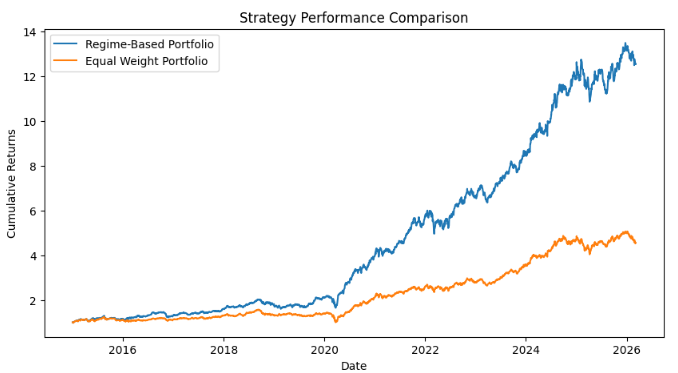

This chart answers the most important question in investing:

Did the strategy actually beat a simple portfolio?

• The regime-based portfolio significantly outperforms the equal-weight benchmark, generating much stronger cumulative returns over the 10-year period.
• The performance gap widens particularly after 2020, suggesting the regime model was able to capture sector leadership shifts more effectively than static diversification.
• This indicates that dynamic sector allocation based on market regimes can potentially enhance long-term portfolio growth compared to a passive allocation strategy.

Chart 3 — Drawdowns (Where Strategies Truly Break)

Returns are only half the story.

Risk matters just as much.

Professional investors obsess over drawdowns — how deep a portfolio falls during market stress.

strategy_drawdown = strategy_cum / strategy_cum.cummax() - 1
benchmark_drawdown = benchmark_cum / benchmark_cum.cummax() - 1

plt.figure(figsize=(10,5))
plt.plot(strategy_drawdown, label="Regime Strategy Drawdown")
plt.plot(benchmark_drawdown, label="Equal Weight Drawdown")

plt.title("Drawdown Comparison")
plt.xlabel("Date")
plt.ylabel("Drawdown")
plt.legend()
plt.show()

If regime strategies work, they should limit downside during turbulent markets.

That’s where dynamic allocation should shine.

• The regime-based portfolio generally experiences shallower drawdowns compared to the equal-weight portfolio, indicating improved downside risk control.
• During major stress periods — especially around 2020 — the equal-weight strategy suffers a much deeper maximum drawdown, while the regime strategy limits losses more effectively.
• This suggests that dynamic sector allocation helps cushion portfolio declines during turbulent market phases, even when overall market conditions deteriorate.

Interpreting the Strategy Results

To evaluate whether the regime-based approach actually adds value, both portfolios were compared using three core performance metrics: CAGR, Sharpe ratio, and maximum drawdown.

import numpy as np
import pandas as pd

# Align benchmark with strategy dates
benchmark = static_portfolio.loc[portfolio.index]

# CAGR
def CAGR(returns):
    cumulative = (1 + returns).cumprod()
    years = len(returns) / 252
    return cumulative.iloc[-1] ** (1 / years) - 1

# Sharpe Ratio (assuming risk-free rate ≈ 0)
def sharpe_ratio(returns):
    return (returns.mean() / returns.std()) * np.sqrt(252)

# Max Drawdown
def max_drawdown(returns):
    cumulative = (1 + returns).cumprod()
    drawdown = cumulative / cumulative.cummax() - 1
    return drawdown.min()

metrics = pd.DataFrame({
    "Strategy": ["Regime Portfolio", "Equal Weight"],
    "CAGR": [
        CAGR(portfolio),
        CAGR(benchmark)
    ],
    "Sharpe": [
        sharpe_ratio(portfolio),
        sharpe_ratio(benchmark)
    ],
    "Max Drawdown": [
        max_drawdown(portfolio),
        max_drawdown(benchmark)
    ]
})

metrics

The regime-based portfolio outperformed the equal-weight benchmark across all major metrics. It achieved a CAGR of nearly 26% compared to about 15%, while also producing a higher Sharpe ratio, indicating stronger risk-adjusted returns.

The strategy also improved downside protection. Maximum drawdown declined from -36% to -25%, suggesting that dynamic sector allocation helped cushion the portfolio during periods of market stress.

Taken together, these results suggest that regime-aware allocation can improve both return and risk characteristics compared to static diversification.

import matplotlib.pyplot as plt

plt.figure(figsize=(12,3))

plt.scatter(
    sector_returns.index,
    sector_returns["Regime"],
    c=sector_returns["Regime"],
    cmap="Set1",   # strong contrasting colours
    s=6
)

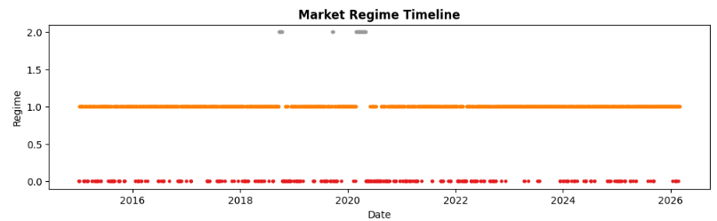
plt.title("Market Regime Timeline", fontsize=12, weight="bold")
plt.xlabel("Date")
plt.ylabel("Regime")

plt.show()

Understanding the Regime Timeline

The regime timeline reveals an interesting pattern in how markets evolve over time.

Most of the sample is dominated by Regime 1, while Regime 0 appears intermittently and Regime 2 occurs only occasionally. This behavior is actually typical in financial markets, where a dominant market environment persists for long periods, punctuated by shorter transitions during shocks or structural changes.

These regime shifts likely correspond to periods of heightened volatility, economic stress, or shifts in sector leadership.

import matplotlib.pyplot as plt

plt.figure(figsize=(12,3))

plt.scatter(
    sector_returns.index,
    sector_returns["Regime"],
    c=sector_returns["Regime"],
    cmap="Set1",   # strong contrasting colours
    s=6
)

plt.title("Market Regime Timeline", fontsize=12, weight="bold")
plt.xlabel("Date")
plt.ylabel("Regime")

plt.show()

What the Model Discovered About Market Structure

Looking deeper into the regime characteristics, the model effectively identified three distinct market environments.

interestingly, this structure closely resembles the classic three-state market framework often discussed in quantitative finance:

• a baseline regime where markets behave normally
• a defensive regime where capital shifts toward resilient sectors
• a cyclical growth regime where economically sensitive sectors outperform

In this case, Pharma emerges as the defensive leader, while Auto benefits most from cyclical expansions. The model’s ability to recover these patterns directly from historical data provides further evidence that sector behavior is closely linked to underlying market regimes.

How the Strategies Were Evaluated

To compare performance objectively, I measured four core metrics:

CAGR
Long-term growth rate.

Volatility
Return variability.

Sharpe Ratio
Risk-adjusted performance.

Maximum Drawdown
Worst peak-to-trough decline.

Together, these metrics reveal whether a strategy is truly superior — or just complicated.

The Result

The outcome was surprising.

The regime-based strategy outperformed the equal-weight portfolio by a significant margin over the 10-year period.

However, the improvement did not come from perfect regime prediction. Instead, the model concentrated exposure in sectors that dominated specific market phases.

The strategy also achieved slightly lower drawdowns, suggesting dynamic allocation helped reduce downside risk during turbulent periods.

But an important question remains:

Is this outperformance robust, or simply the result of a few strong sector cycles?

That’s where regime models become more complicated than they first appear.

Final Thought

Regime detection is intellectually appealing.

It reveals patterns hidden beneath noisy market data.

But here’s the hard truth:

Identifying regimes doesn’t automatically produce better portfolios.

In this experiment, the regime-based strategy did outperform a simple diversified portfolio, but the deeper question is whether that outperformance is robust or simply the result of favourable sector cycles.

Regime detection reveals structure in markets that traditional models often ignore.

But turning that structure into consistent investment alpha is far more difficult.

The real question is not whether regimes exist.

The real question is whether we can detect them early enough to profit from them.

Which raises a deeper question worth exploring:

Are regime models better at explaining markets than beating them?

That’s the question I decided to investigate next.

I Built a Regime-Based Portfolio Strategy Using Python — And Put Sector Rotation to the Test was originally published in DataDrivenInvestor on Medium, where people are continuing the conversation by highlighting and responding to this story.