Building an Autonomous Robot Car from First Principles: Transistors, H-Bridges, Ultrasonic Physics, and the Engineering Behind a Machine That Thinks for Itself
A complete engineering build log covering DC motor theory, H-bridge topology, pulse-width modulation, embedded state machines, and the physical assembly of a two-wheel differential drive robot.
There is a particular kind of satisfaction that comes from placing a small machine on the floor, switching it on, and watching it navigate the world without any instruction from you. Not because it is running some impressive neural network or communicating with a cloud server; but because you wired it up yourself, you wrote the code yourself, and somewhere inside that tangle of jumper wires and screw terminals, the physics you studied in a lecture hall is doing something real and tangible. The robot moves. It detects a wall. It reverses, turns, and carries on. It does exactly what you told it to do; and you understand, at every level of abstraction, precisely why.
That is what this build log is about.
This is not a tutorial in the traditional sense. I am not going to tell you to “connect pin A to pin B and upload the code.” I am going to start at the level of electrons moving through a conductor and build upward, layer by layer, until we arrive at a fully functioning autonomous obstacle-avoidance robot car. Every component will be explained from the ground up. Every design decision will be justified. Every line of code will be understood rather than simply copied.
I built this robot as part of my ongoing work in embedded systems and robotics during my engineering studies at UEA. It sits alongside a more advanced platform I am currently developing; a custom 3D-printed chassis with a more sophisticated electronics stack and a richer software architecture. That second robot is not finished, so it will appear only briefly here as context for where this line of work is heading. The focus of this piece is entirely on the simpler two-wheel platform: the one that taught me almost everything I needed to know before attempting anything more ambitious.
For the full-code, visit my GitHub: https://github.com/MooMooCow29/Building-an-Arduino-Robot-Car

Let us begin.
Part One: The Physics Underneath Everything
Before a single wire is connected, it is worth spending time with the physics that make this project possible. Engineering education has a tendency to present components as black boxes with defined inputs and outputs. That is a useful abstraction for getting things done quickly; but it is a terrible foundation for understanding why things go wrong, or how to make them better. So we start here.

Voltage, Current, and Resistance: The Foundation
Voltage is a measure of electric potential difference. It is the pressure that drives charge carriers through a conductor; analogous, at the risk of overusing the analogy, to the pressure that drives water through a pipe. We measure it in volts, named after Alessandro Volta.
Current is the rate of flow of that charge. One ampere is one coulomb of charge passing a point per second. In a copper wire, the charge carriers are free electrons; and when a potential difference is applied across the wire, those electrons drift in a net direction, constituting a current.
Resistance is the opposition to that flow. It arises from collisions between electrons and the lattice structure of the conductor. Georg Simon Ohm described the relationship between these three quantities in what is now the most fundamental equation in circuit analysis:
V = I × R

This equation is deceptively simple. Every calculation in this project flows from it. When the Arduino Uno outputs a HIGH signal on one of its GPIO pins, it provides 5 volts. When you connect a load to that pin, Ohm’s Law governs how much current flows. The Arduino can source or sink a maximum of 40 milliamps from any single digital pin; exceed that, and you begin permanently damaging the output driver transistor inside the chip. A DC motor at stall draws several hundred milliamps. This is why you cannot drive a motor directly from an Arduino pin; and this is why the L298N motor driver module exists.
Power and Energy: Why Battery Life Matters
Power is the rate of energy transfer. It is measured in watts, and calculated as:
P = V × I
A motor running at 6 volts and drawing 300 milliamps consumes 1.8 watts. Over one hour, that is 1.8 watt-hours of energy drawn from the battery. A standard 9-volt alkaline battery holds approximately 550 milliamp-hours of charge. Running both motors simultaneously, powering the Arduino, and occasionally firing the ultrasonic sensor draws somewhere in the region of 400 to 600 milliamps from the battery at moderate speed. That gives a runtime of roughly 50 minutes to an hour per battery; which sounds short, but is entirely reasonable for a test platform.
The practical implication of this is that battery selection is not a trivial decision. Alkaline cells are cheap, widely available, and require no special charger; but they sag significantly under load, their voltage dropping noticeably as they deplete. A lithium polymer (LiPo) pack provides a flatter discharge curve and far higher energy density for the same weight. It is the standard upgrade for any robotics platform that needs longer endurance or more consistent motor performance; and it is one of the first changes I intend to make on the more advanced platform.

The DC Motor: Electromagnetic Energy Conversion
A direct-current motor is a device that converts electrical energy into rotational mechanical energy through electromagnetic induction. Understanding how it works at the level of physics is essential for understanding why it behaves the way it does under different control strategies.
Inside the motor casing, a wound rotor; sometimes called the armature; sits inside a static magnetic field produced by permanent magnets attached to the stator. When current flows through the rotor windings, each current-carrying conductor experiences a force. This force is described by the Lorentz force law:
F = I L × B
Where F is the force on the conductor, I is the current, L is the length of the conductor in the field, and B is the magnetic flux density. The direction of the force is perpendicular to both the current and the magnetic field; which is what causes the rotor to rotate rather than simply translate.
As the rotor turns, the commutator (a segmented copper ring) and the brush assembly (spring-loaded carbon contacts) periodically reverse the direction of current in each winding. This reversal is timed to maintain a continuous torque in one direction regardless of rotor position; which is the ingenious mechanical trick that makes a brushed DC motor self-sustaining in its rotation.
Two key relationships govern motor behaviour in steady state. First, speed is approximately proportional to applied voltage above the back-EMF threshold. The back-EMF (electromotive force) is a voltage generated by the spinning rotor that opposes the supply voltage; it increases with speed and is the reason motor current drops as the motor spins up. Second, torque is approximately proportional to armature current. This means that when a motor stalls (rotation stops under heavy load), current rises sharply; which is why stalled motors get hot and why overcurrent protection matters.
The TT gear motors used in this build include a 1:48 planetary gearbox. This trades output speed for output torque by a factor of 48. The bare motor might spin at 9,600 RPM; the output shaft delivers 200 RPM with 48 times the torque. That additional torque is what allows the robot to actually move its own weight across a carpeted floor rather than spinning its wheels fruitlessly.

Transistors and Semiconductor Switching
The transistor is the fundamental building block of modern electronics. A bipolar junction transistor (BJT) has three terminals: the base, the collector, and the emitter. A small current flowing into the base enables a much larger current to flow from collector to emitter. The ratio of these currents is the current gain, denoted h_FE or β, and is typically in the range of 50 to 300 for common signal transistors.
This amplification property is precisely what allows a microcontroller to control a motor. The Arduino GPIO pin cannot supply enough current to run a motor directly; but it can supply enough base current to turn on a transistor, which then allows the motor’s full current to flow through its own separate supply path. The transistor acts as an electronically controlled switch; and that switch is the basis of every motor controller ever built.
Modern high-power applications use MOSFETs (metal-oxide-semiconductor field-effect transistors) rather than BJTs, because MOSFETs are voltage-controlled (rather than current-controlled), switch faster, and have lower on-state resistance. The L298N uses bipolar transistors internally; which limits its efficiency somewhat, but makes it robust and easy to use.
The H-Bridge: Reversibility Through Topology
A single transistor can only switch current on or off; it cannot reverse the direction of current through a load. To reverse a DC motor, you need to reverse the polarity of the supply voltage across its terminals. The H-bridge circuit achieves this electronically without any mechanical switching.
The name comes from the schematic shape of the circuit: four switches arranged in an H, with the motor connected across the middle. By closing different pairs of switches, current can be made to flow through the motor in either direction:
When switches S1 and S4 are closed (with S2 and S3 open), current flows from left to right through the motor. The motor rotates forward. When S2 and S3 are closed (with S1 and S4 open), current flows from right to left. The motor rotates backward. Close S1 and S2 simultaneously, or S3 and S4 simultaneously, and you create a direct short circuit across the power supply; a catastrophic condition called shoot-through that can destroy the transistors and the battery in milliseconds. Competent H-bridge implementations include logic to prevent this; but understanding why it is dangerous helps you appreciate why the rule exists.
The L298N contains two complete H-bridges in a single package; one for each motor. This is why it is called a dual H-bridge motor driver.
Pulse-Width Modulation: Speed Control Without Wasted Heat
If the only thing an H-bridge could do was run a motor at full speed or stop it, it would be of limited use for a robot that needs to navigate smoothly. Speed control is achieved through pulse-width modulation; a technique that turns the motor supply on and off at high frequency and varies the proportion of time it is on.
The duty cycle is the fraction of each cycle during which the signal is HIGH, expressed as a percentage. A duty cycle of 100% delivers full voltage to the motor continuously. A duty cycle of 50% delivers full voltage for half the cycle and zero for the other half. Because the inductance of the motor windings acts as a low-pass filter; smoothing the pulsed voltage into an approximately constant average; the motor experiences the 50% duty cycle as though it were running at half voltage. It spins at roughly half speed.
The Arduino Uno implements hardware PWM on six of its pins: 3, 5, 6, 9, 10, and 11. The analogWrite() function accepts a value between 0 and 255, where 0 is 0% duty cycle and 255 is 100%. This 8-bit resolution gives 256 discrete speed levels per motor; which is more than sufficient for the kind of control needed in this project.
A critical advantage of PWM over resistive speed control is efficiency. A series resistor wastes energy as heat; the motor voltage drops, but the wasted energy goes nowhere useful. PWM wastes almost no energy in the switching process itself; the transistors are either fully on (very low resistance; very low power dissipation) or fully off (zero current; zero power dissipation). The motor gets the full supply voltage during the ON phase; and the average determines speed. This is why every serious motor controller uses PWM rather than resistive control.
Part Two: Understanding Every Component
The Arduino Uno R3
The Arduino Uno is built around the Atmel ATmega328P microcontroller; an 8-bit AVR RISC processor clocked at 16 MHz. Its modest specification belies its capability for embedded control tasks:
Attribute Value Architecture 8-bit AVR RISC Clock 16 MHz Flash 32 KB (0.5 KB bootloader) SRAM 2 KB EEPROM 1 KB Digital I/O 14 pins PWM outputs 6 pins Analogue inputs 6 channels (10-bit ADC) Operating voltage 5 V Recommended input 7–12 V Max GPIO current 40 mA per pin
What makes the Arduino Uno interesting from an engineering perspective is not the MCU itself; it is the surrounding ecosystem. The USB interface is handled by a separate ATmega16U2 chip (or a CH340G on cheaper clones), which enumerates as a virtual COM port on the host computer. This allows the bootloader to receive new firmware over USB without needing a dedicated hardware programmer. The bootloader sits in the upper 0.5 KB of flash and runs for approximately 1 to 2 seconds at reset, listening for incoming serial data. If none arrives, it jumps to the start of the user sketch. This entire mechanism is invisible to the user; but understanding it helps explain why there is always a brief pause after pressing reset before the program runs.
The onboard 5-volt linear regulator converts the barrel jack or VIN input (7 to 12 volts) to a regulated 5-volt rail for the MCU and peripherals. “Linear” regulator means it dissipates the voltage difference as heat; a 9-volt input with a 200-milliamp load produces (9−5) × 0.2 = 0.8 watts of heat in the regulator. This is manageable; but powering motor drivers through this regulator would quickly overheat it. In this build, the L298N is powered directly from the battery and feeds 5 volts back to the Arduino; reversing the usual power flow and bypassing the Uno’s onboard regulator entirely.
The Arduino IDE presents this hardware through a C++ abstraction layer that hides the register-level complexity of the AVR peripherals. Functions like pinMode(), digitalWrite(), and analogWrite() map to specific bit manipulations of the MCU's internal registers. This is enormously helpful for getting started; but it is worth knowing that behind analogWrite(9, 180) lies a Timer 1 configuration that sets a specific OCR1A compare register value and enables the non-inverting PWM output mode on OC1A. The abstraction is leaky in some useful ways; understanding it makes you a better embedded programmer.
The L298N Dual H-Bridge Motor Driver Module
The L298N is a monolithic integrated circuit manufactured by STMicroelectronics. The module form factor; a small PCB carrying the L298N chip alongside decoupling capacitors, a 5-volt onboard regulator, screw terminals for motor connections, and pin headers for logic signals; is the version commonly used in hobby robotics.
The chip contains two fully independent H-bridge circuits, each capable of driving up to 2 amperes continuously. The logic supply (VSS) accepts 5 volts from the Arduino; the motor supply (VS) accepts 5 to 46 volts directly from the battery. This separation of logic and power supplies is fundamental: the Arduino’s sensitive 5-volt logic circuitry is isolated from the noisy, high-current motor supply. Without this isolation, the voltage spikes generated by motor switching (caused by the inductance of the motor windings; which resists sudden changes in current) would couple into the logic supply and cause the Arduino to behave erratically or reset.
The enable pins (ENA and ENB) act as the PWM input for each channel. When ENA is driven with a PWM signal, the H-bridge modulates the average voltage delivered to Motor A accordingly. When ENA is pulled HIGH (by connecting it to 5 volts via the onboard jumper), the motor runs at full speed and cannot be speed-controlled. Removing the jumper and connecting ENA to an Arduino PWM pin gives full variable-speed control; which is what this build does.
One important limitation of the L298N is its voltage drop. The internal bipolar transistors each drop approximately 1 volt when conducting; with two transistors in series in the current path, the total drop across the H-bridge is roughly 2 volts. A 9-volt battery supply therefore delivers approximately 7 volts to the motors. As the battery discharges and its terminal voltage drops toward 7 volts, the motors receive only 5 volts and their speed noticeably reduces. This is a known weakness of the L298N topology; MOSFET-based drivers (such as the DRV8833 or TB6612FNG) have on-state resistances of tens of milliohms rather than 1-volt drops, and are far more efficient. For a first build, the L298N is acceptable. For the advanced platform, a MOSFET driver is the correct choice.
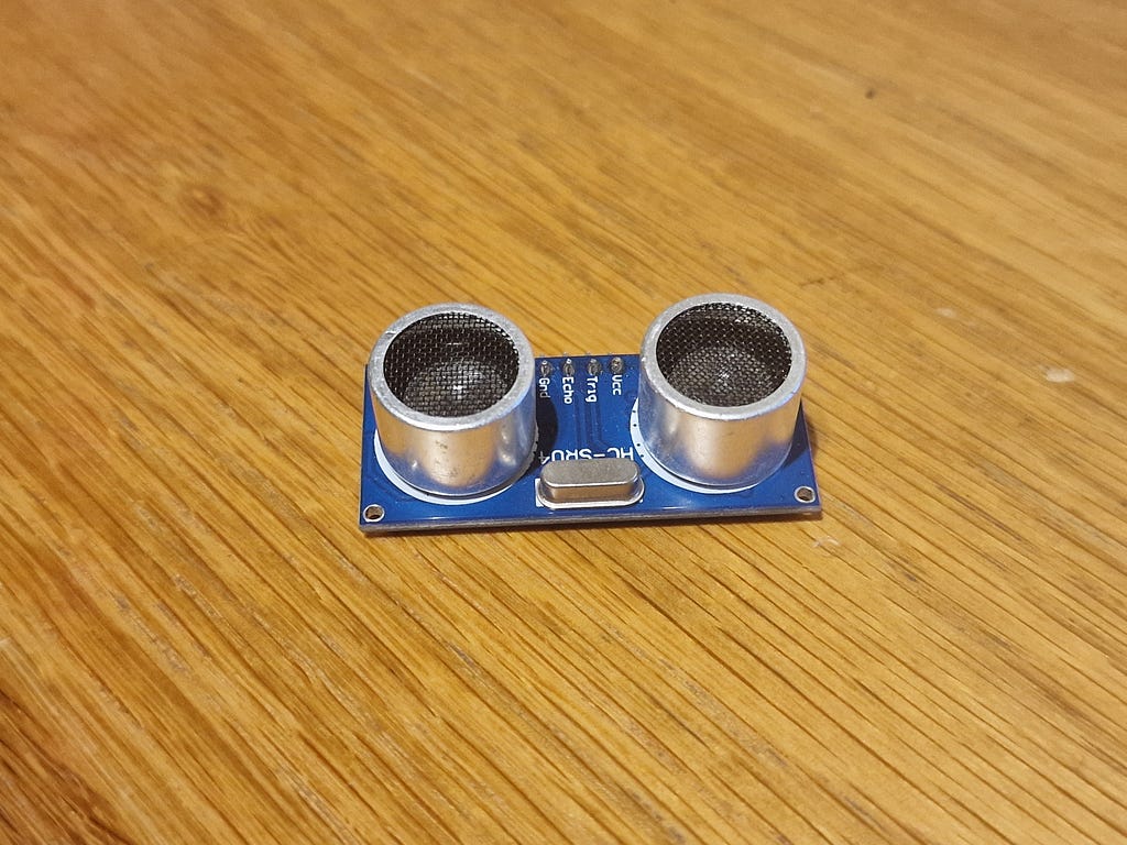
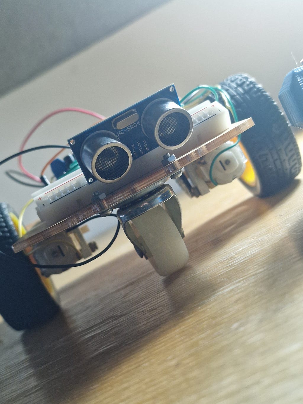
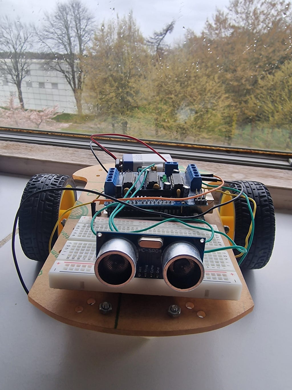
The HC-SR04 Ultrasonic Distance Sensor
The HC-SR04 is a ubiquitous sensor in hobbyist robotics, and for good reason: it is cheap, robust, easy to interface, and accurate enough for obstacle detection. It operates on the time-of-flight principle: a burst of 40-kilohertz ultrasonic sound is transmitted from one transducer, bounces off a surface, and is received by the second transducer. The time between transmission and reception is proportional to the distance to the surface.
The physics here is straightforward. The speed of sound in dry air at 20°C is approximately 343 metres per second; equivalently, 0.0343 centimetres per microsecond. Since the pulse must travel to the obstacle and back, the round-trip distance is:
round-trip distance = 0.0343 cm/µs × time_in_µs
one-way distance    = (0.0343 × time_in_µs) / 2
                    = time_in_µs / 58.3
                    ≈ time_in_µs / 58
This division by 58 is the conversion formula used in virtually every HC-SR04 implementation. The Arduino’s pulseIn() function measures the duration of the Echo pin's HIGH pulse in microseconds; dividing by 58 gives distance in centimetres.
A few practical notes that the datasheet does not make immediately obvious. The sensor has a blind zone below approximately 2 centimetres; objects closer than this cannot be detected because the echo return overlaps with the outgoing trigger pulse. The nominal maximum range of 400 centimetres is achievable only with a large flat reflective surface directly in front of the sensor; real-world maximum range against typical obstacles is closer to 150 to 200 centimetres. The radiation pattern is a cone of approximately 15 degrees half-angle; this means the sensor will detect objects that are not directly ahead, which can cause unexpected behaviour in cluttered environments. And the sensor should be triggered no more than 40 times per second (once every 25 milliseconds) to allow the ultrasonic echoes from each measurement to decay before the next trigger is sent; triggering faster than this produces spurious readings as old echoes are mistaken for new ones.
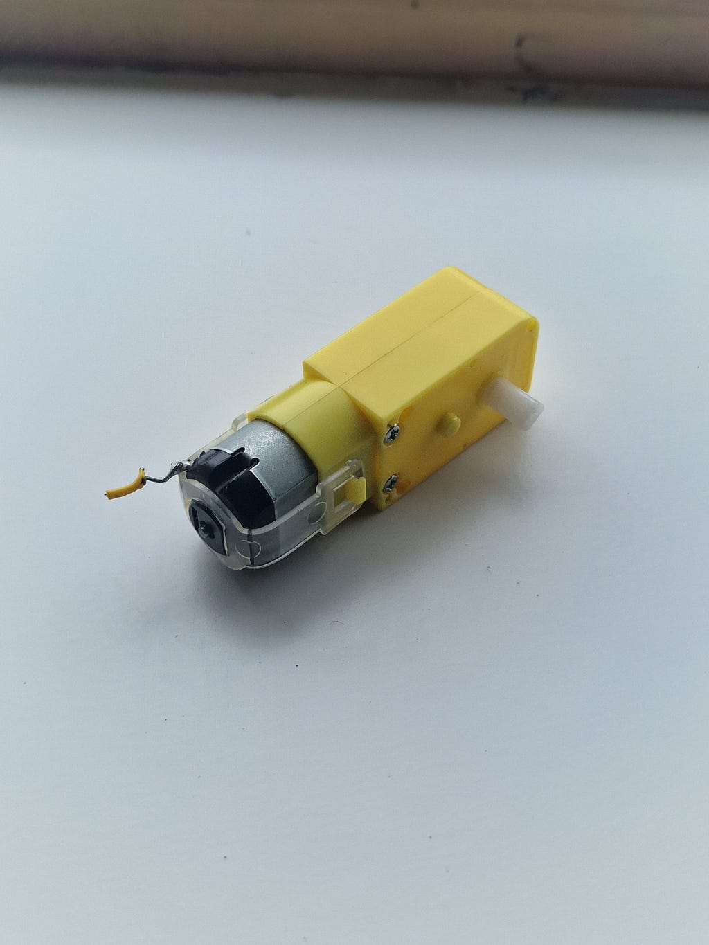
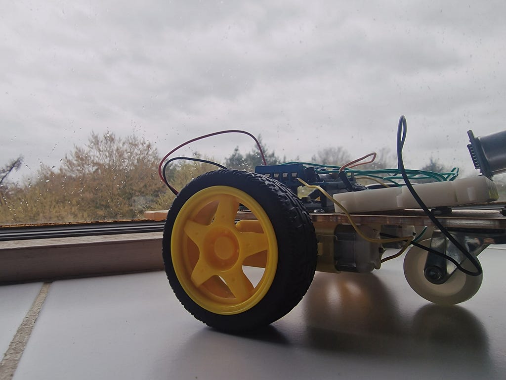
The TT Gear Motors
The yellow TT-format gear motors are the workhorses of entry-level robotics. Inside the plastic housing sits a small brushed DC motor; the type we analysed in the previous section. The output shaft passes through a 1:48 gearbox; either a planetary type or a simple spur gear train depending on the manufacturer.
Rated voltage is 3 to 6 volts. At 6 volts with no mechanical load, the output shaft rotates at approximately 200 RPM. Stall current (maximum current when the shaft is prevented from rotating) is approximately 800 milliamps to 1.2 amperes per motor; this is the peak current demand that the power supply and motor driver must be capable of supplying.
The wheels attached to these motors are 65 millimetres in diameter, giving a circumference of π × 65 ≈ 204 millimetres. At 200 RPM, the linear ground speed of the robot is 200 × 204 mm/min = 40,800 mm/min ≈ 0.68 m/s. In practice, accounting for the L298N voltage drop, battery sag, and mechanical losses in the gearbox, the actual top speed is closer to 0.4 to 0.5 metres per second. At the drive speed used in the firmware (a PWM value of 180 out of 255; approximately 70% duty cycle), forward speed is roughly 0.3 metres per second. This is fast enough to be interesting and slow enough to stop before hitting most obstacles at the 30-centimetre threshold.
Part Three: The Chassis and Physical Assembly
Choosing the Differential Drive Architecture
The differential drive architecture; also known as tank drive or skid steer; is the simplest and most common drive system for ground robots. Two independently powered wheels share a common axis. A third unpowered wheel (or caster) provides the additional ground contact needed for stability.
Steering is achieved entirely by varying the relative speeds and directions of the two drive wheels:
- Both wheels forward at equal speed: the robot moves straight ahead.
- Both wheels backward at equal speed: the robot moves straight backward.
- Left wheel forward, right wheel stopped: the robot curves to the right (pivots around the right wheel).
- Left wheel forward, right wheel backward at equal speed: the robot spins in place to the right.
There is no dedicated steering mechanism. There is no servo, no rack and pinion, no Ackermann geometry. The simplicity of this arrangement is both its greatest strength (fewer components to fail; simpler firmware; minimal mechanical complexity) and its greatest weakness (no odometric accuracy; wheels skid during turns rather than rolling cleanly; heading control requires encoder feedback for precision). For obstacle avoidance, these weaknesses are entirely acceptable.
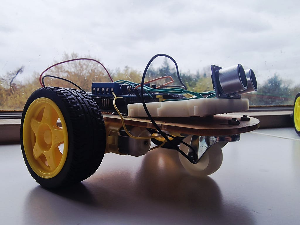
The MDF Chassis
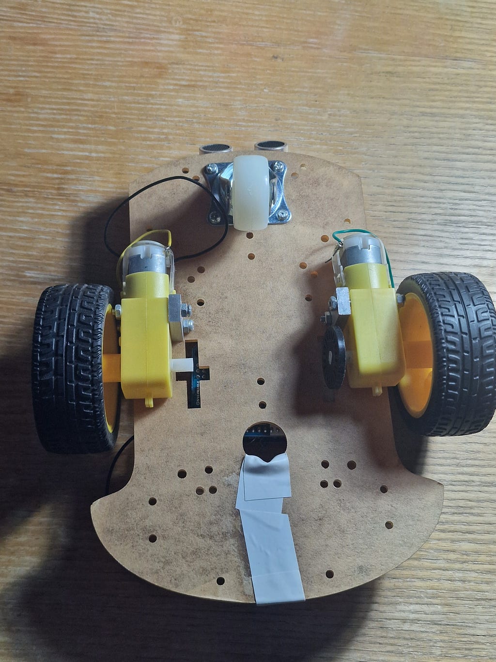
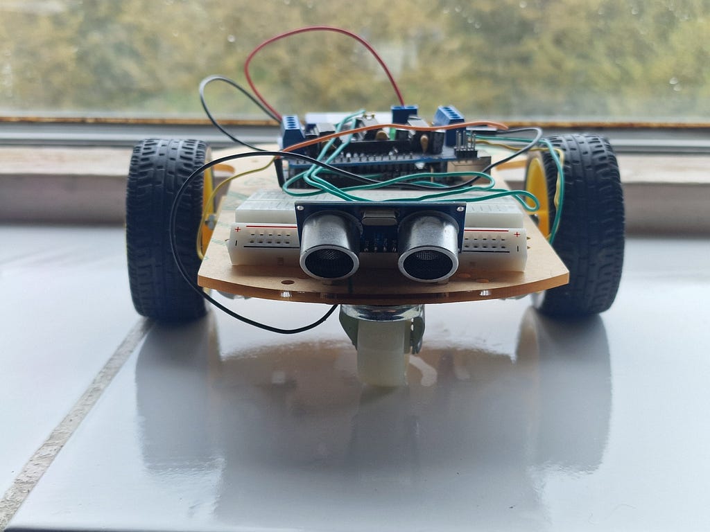
The chassis is a laser-cut medium-density fibreboard platform with a rounded rectangular profile and a forward extension that houses the caster wheel mount. MDF is a sensible choice for a first build: it is dimensionally stable, easy to drill, and electrically non-conductive. A metallic chassis would require careful insulation beneath every component to prevent short circuits between PCB solder joints and the chassis surface; MDF requires no such precaution.
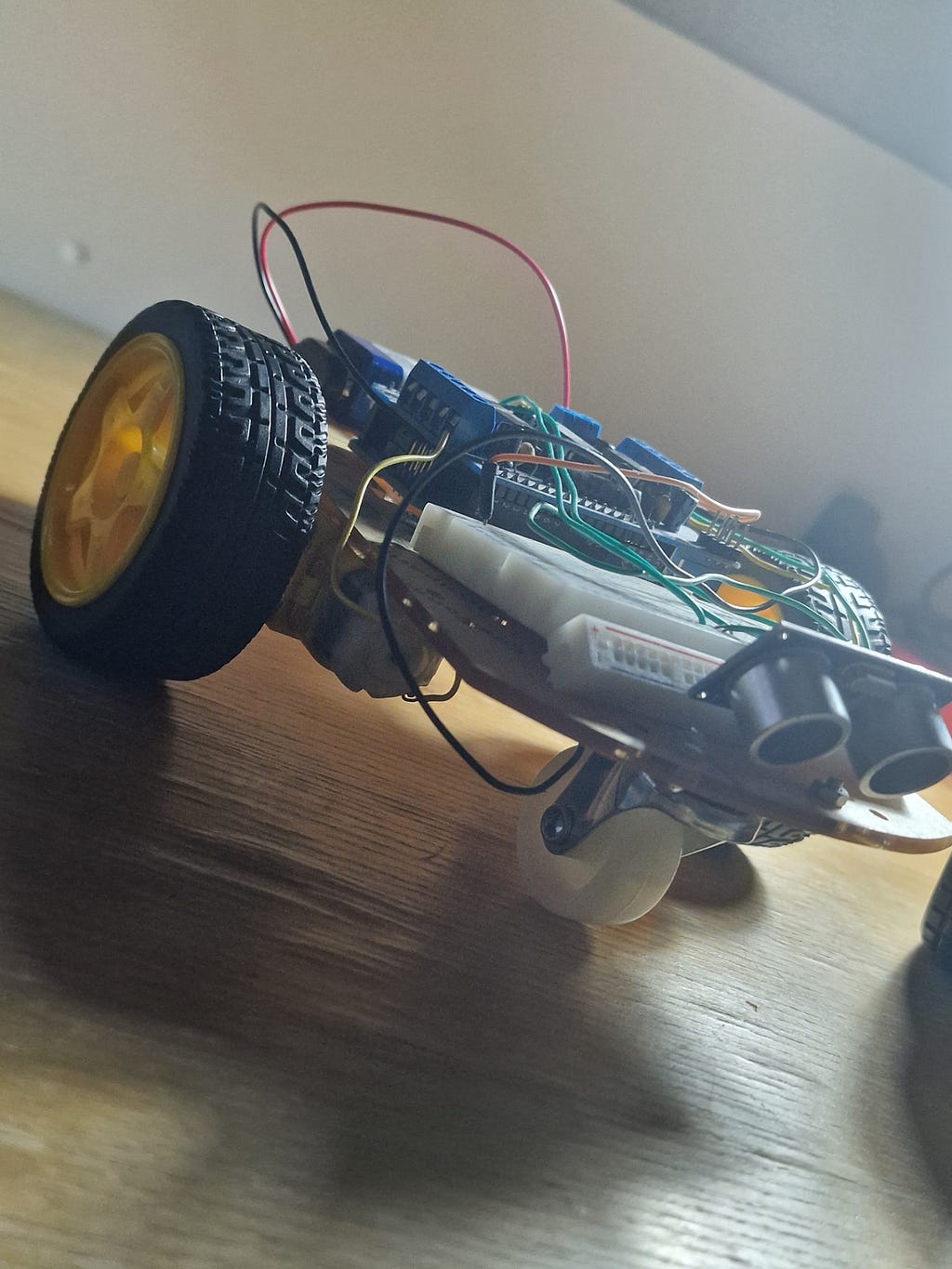
The two drive motors mount to the rear of the chassis from below using yellow plastic motor brackets, each secured with two M3 bolts. The swivel caster mounts at the front centre with four M3 bolts and provides a frictionless forward support point. The three contact points; the two drive wheels and the caster; define a stable support plane (a tripod arrangement that cannot rock) regardless of small surface irregularities.
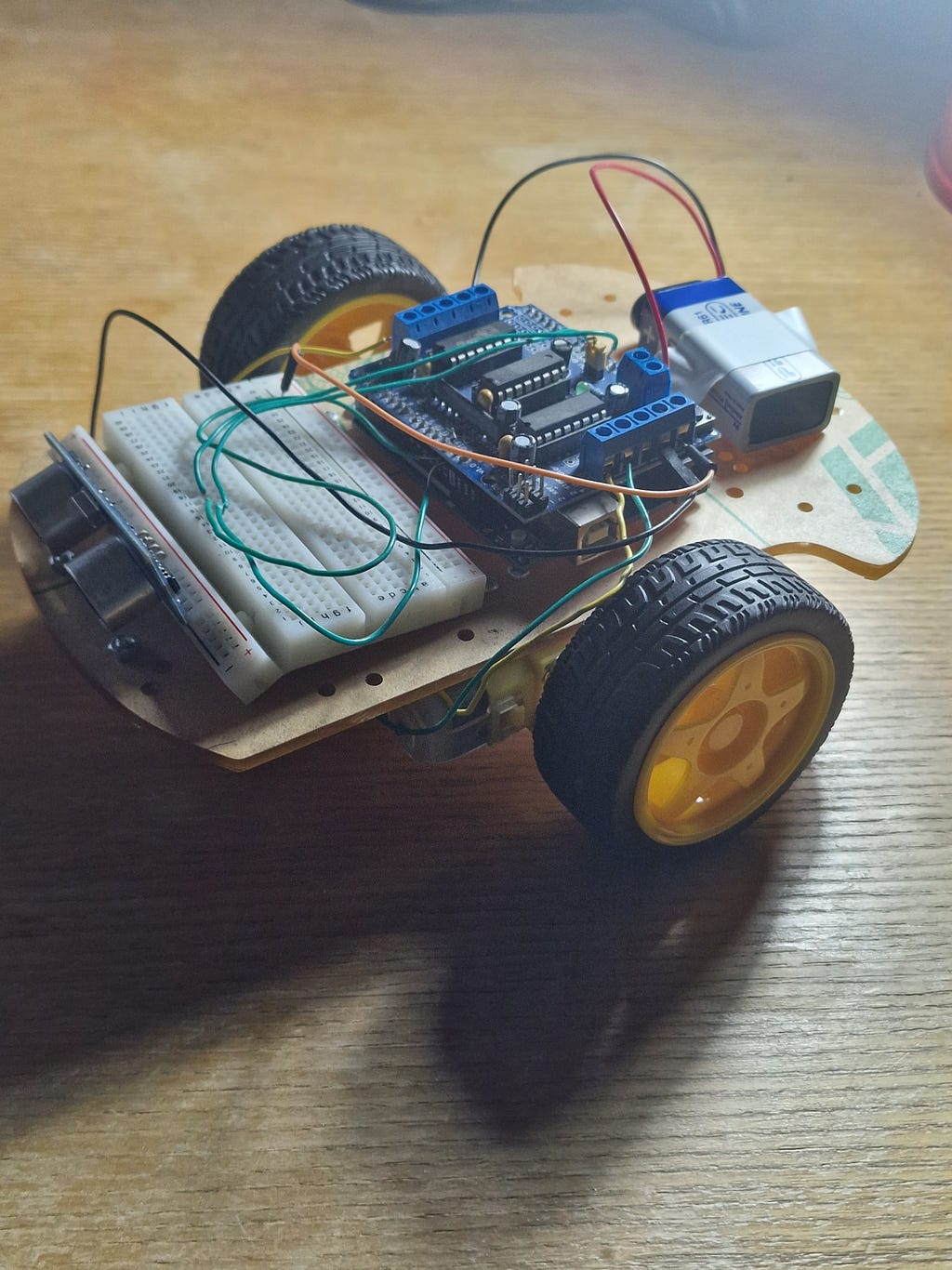
Electronics mount on the upper surface of the chassis using M3 standoffs to create a 10-millimetre air gap between each PCB’s solder joints and the MDF. The Arduino Uno sits roughly in the centre of the chassis. The L298N module sits near the rear motors to minimise the length of the high-current motor wires; long motor wires act as antennae, radiating electromagnetic noise that can corrupt sensor readings and even cause the Arduino to reset. The breadboard is fixed to the front of the chassis using its self-adhesive pad and carries the HC-SR04 sensor.
The 9-volt battery is held to the underside of the chassis with hook-and-loop tape; allowing quick removal for replacement without disturbing any wiring.
Motor Mirroring: The Most Commonly Missed Detail
There is one mechanical fact about differential drive robots that catches almost every first-time builder by surprise. Because the left and right motors are mounted facing opposite directions on the chassis (one faces left; the other faces right), “forward” rotation for the left motor corresponds to “backward” rotation for the right motor when judged purely by the direction of shaft spin.
To drive the robot forward, the left motor must spin clockwise (when viewed from its output shaft end) while the right motor must spin counter-clockwise. If you apply the same electrical polarity to both motors, the robot will spin in place rather than move forward. The firmware handles this by intentionally inverting the direction pins of one motor relative to the other; setting IN1=HIGH/IN2=LOW for the left motor (forward) while setting IN3=LOW/IN4=HIGH for the right motor (also physically forward). This inversion is encapsulated inside the motors.cpp module; higher-level code never needs to think about it.
If, after assembly, the robot spins in place when commanded to go forward, the fix is simple: swap the wire pair for one motor at the L298N’s screw terminals. Alternatively, invert that motor’s IN3/IN4 values in the firmware. Either approach achieves the same result.
Part Four: Wiring It All Together
The Power Architecture
Sound power distribution is one of the most important and most neglected aspects of robot wiring. The rule is simple: every component that shares electrical ground must have a physical wire connecting its GND pin to the same common ground node. Failing to do this causes reference voltage differences between subsystems; which manifests as erratic behaviour that is infuriatingly difficult to diagnose because it does not have an obvious single cause.
In this build, the power architecture is as follows:
The 9-volt battery positive terminal connects to the L298N’s VS (motor supply) terminal. The battery negative terminal connects to the L298N’s GND terminal. The L298N’s onboard 5-volt regulator (enabled when the 5V jumper is present) produces a regulated 5-volt output that connects to the Arduino’s 5V pin; bypassing the Uno’s own regulator. The Arduino’s 5V pin feeds the HC-SR04’s VCC and the L298N’s VSS (logic supply). The Arduino’s GND pin connects to the L298N’s GND terminal and to the HC-SR04’s GND pin.
The common ground net; battery negative, L298N GND, Arduino GND, HC-SR04 GND; is the most critical connection in the entire circuit. Without it, the logic-level signals on the IN1 through IN4 pins are being referenced against a floating potential, and the L298N will ignore them or respond to them unpredictably. In my own testing, omitting the common ground connection produced a robot whose motors would spin apparently at random; sometimes responding to commands, sometimes not, changing behaviour whenever the battery voltage fluctuated. Adding a single wire from Arduino GND to L298N GND resolved it instantly. This is not a subtle lesson.
Signal Wiring
The six control signals from the Arduino to the L298N are standard 5-volt digital and PWM connections. ENA on pin 9 and ENB on pin 6 are PWM outputs. IN1 on pin 8, IN2 on pin 7, IN3 on pin 5, and IN4 on pin 4 are standard digital outputs. The HC-SR04 Trig connects to pin 13 and Echo to pin 12.
One thing worth noting about the Echo pin: the HC-SR04 outputs a 5-volt pulse, and the Arduino’s digital inputs accept 5-volt signals; so no level shifting is required. Had this build used a 3.3-volt microcontroller (the ESP32, for example, which runs at 3.3-volt logic), a voltage divider on the Echo line would be mandatory to protect the input pin from the 5-volt signal.
Wiring Hygiene
Physical wiring quality has a direct effect on electrical reliability. A few principles that make a significant difference:
Keep motor power wires (the red and black wires connecting battery to L298N, and the wires from L298N to motors) physically separated from signal wires. Motor wires carry switching current at high frequency; the rapid current changes generate magnetic fields that can induce voltage spikes in adjacent signal wires through mutual inductance. In serious designs, shielded cable or twisted pairs are used; in this build, simply routing the power and signal wires on opposite sides of the chassis is sufficient.
Keep motor wires short. Longer wires have greater inductance; which means larger voltage spikes during switching. The motor wires in this build are approximately 10 centimetres long; more than adequate.
Add a 100-microfarad electrolytic capacitor across the battery terminals, placed physically close to the L298N VS and GND terminals. Motor inrush current (the brief surge of current when a motor starts from rest) can momentarily collapse the battery terminal voltage; the capacitor acts as a local energy reservoir that absorbs this spike and prevents it from propagating into the logic supply and resetting the Arduino.
Part Five: The Firmware in Depth
Why Architecture Matters in Embedded Code
It is tempting, when writing code for a small microcontroller, to view software architecture as a luxury that only large projects need. This is wrong; and on an embedded system, the consequences of poor architecture are particularly visible because the hardware reflects software quality directly in physical behaviour.
The most common mistake in beginner robotics code is the heavy use of delay(). The Arduino delay() function burns CPU cycles in a busy-wait loop until the specified number of milliseconds has elapsed. During this time, the processor executes no other instructions. It cannot read the sensor. It cannot update the motor commands. It cannot respond to any input whatsoever. For a robot that needs to sense its environment continuously, this is a serious problem: the robot is effectively blind during every delay() call.
The firmware for this build is structured as a non-blocking state machine. The state of the robot (driving forward; stopped; reversing; turning) is stored as an enum variable. Transitions between states are triggered by elapsed time, measured using millis() (which returns the number of milliseconds since the board was powered on) rather than blocking delays. The main loop executes as fast as possible; typically at several thousand iterations per second; and the sensor is read on every iteration. The robot is never blind.
The State Machine
The robot operates in four states:
STATE_FORWARD: Both motors drive forward at DRIVE_SPEED. On every loop iteration, the distance to the nearest obstacle is measured. If it falls below STOP_DISTANCE (30 centimetres), the motors are stopped and the state transitions to STATE_STOP. Otherwise, the robot continues forward.
STATE_STOP: Motors are halted. The firmware waits for STOP_PAUSE_MS (200 milliseconds) to allow the robot to decelerate and settle before the next manoeuvre. After this pause, the state transitions to STATE_REVERSING.
STATE_REVERSING: Both motors drive backward at REVERSE_SPEED. After REVERSE_TIME_MS (400 milliseconds), the motors stop briefly, and the state transitions to STATE_TURNING.
STATE_TURNING: The left motor drives forward and the right motor is stopped; a pivot turn to the right. After TURN_TIME_MS (500 milliseconds), the motors stop and the state returns to STATE_FORWARD.
The elegance of this architecture is that the sensor measurement on every loop iteration continues to be valid even during the reversing and turning phases. If during a reversing manoeuvre the robot were to approach a new obstacle from behind (say, on a cluttered table), the sensor reading would reflect this; and a more sophisticated state machine could react to it. The blind-spot problem of delay-based code is eliminated entirely.
The Complete Firmware
The firmware is split across four files, reflecting good software engineering practice:
config.h contains every tunable constant in the system; speeds, thresholds, pin assignments, and timing values. Nothing is hard-coded in the implementation files. Adjusting robot behaviour requires editing only one file.
motors.h and motors.cpp implement the motor driver abstraction layer. The public API consists of semantic functions: motors_forward(), motors_backward(), motors_turn_right(), motors_spin_right(), motors_brake(), motors_stop(). The internal implementation handles the physical-level detail of IN1/IN2/IN3/IN4 polarity; including the mirror-mounting inversion. No other part of the codebase ever manipulates motor driver pins directly.
ultrasonic.h and ultrasonic.cpp implement the sensor abstraction. ultrasonic_read_cm() returns a distance in centimetres; ultrasonic_read_us() returns the raw echo pulse duration. The conversion formula and timeout handling are encapsulated here.
robot_car.ino contains only the state machine logic and the setup/loop structure. It calls motor and sensor functions by name; it never sets a pin directly. The result is code that reads almost like a specification: “if distance is less than threshold, stop motors, transition to stop state.”
This separation of concerns is the correct way to structure embedded firmware. Each module can be tested independently (the two test sketches in the repository; test_motors.ino and test_ultrasonic.ino; do exactly this). Each module can be replaced or upgraded without touching the others. When the motor driver is eventually upgraded from the L298N to a MOSFET-based driver, only motors.cpp changes; nothing else needs to be touched.
Key Code Sections Explained
The trigger sequence for the HC-SR04 warrants careful explanation because it is a precise timing requirement specified in the datasheet:
digitalWrite(PIN_TRIG, LOW);
delayMicroseconds(2);           // Guarantee a clean low before triggering
digitalWrite(PIN_TRIG, HIGH);
delayMicroseconds(10);          // 10 µs trigger pulse required by datasheet
digitalWrite(PIN_TRIG, LOW);
return pulseIn(PIN_ECHO, HIGH, ULTRASONIC_TIMEOUT_US);
The 2-microsecond low period before the trigger pulse ensures that the Trig pin is genuinely low before the rising edge; without this, if the pin was previously high for any reason, the sensor might not register a valid trigger. The 10-microsecond HIGH pulse is the minimum required by the HC-SR04 datasheet to initiate a measurement cycle. pulseIn() then waits for the Echo pin to go HIGH, measures how long it stays HIGH, and returns that duration in microseconds. The timeout parameter (30,000 microseconds; equivalent to approximately 5 metres) prevents the function from hanging indefinitely if no echo is received.
The motor forward function illustrates the mirror-mounting inversion:
void motors_forward(uint8_t speed) {
  left_forward(speed);    // IN1=HIGH, IN2=LOW
  right_forward(speed);   // IN3=LOW, IN4=HIGH  ← note the inversion
}
The right motor’s internal function sets IN3=LOW and IN4=HIGH; the physical opposite of what you might naively expect; because the right motor is mounted facing the opposite direction to the left motor. This is the kind of detail that belongs in an implementation file rather than scattered throughout the main logic.
Part Six: Testing and Calibration
The Correct Order of Testing
Hardware and software debugging are far easier when done in the right order. The principle is simple: test each subsystem in isolation before integrating them. Do not attempt to debug a system where the motors might be wired backwards AND the sensor might be misread AND the state machine might have a logic error; all simultaneously. Isolate each variable.
Step 1: Motor wiring test. Upload test_motors.ino. This sketch exercises each motor individually in both directions, then both motors together, then turns. Watch the Serial Monitor at 9600 baud and observe whether the physical motor behaviour matches the description. If the left motor runs backward when commanded forward, swap its wire pair at the L298N’s OUT1/OUT2 terminals. If the right motor has the same issue, swap OUT3/OUT4. Do not touch the firmware; resolve motor direction issues at the hardware level.
Step 2: Sensor test. Upload test_ultrasonic.ino. Open the Serial Monitor. Hold your hand at various distances in front of the sensor and verify that the readings track your hand’s position correctly, change smoothly, and stabilise at consistent values. A reading of 999 at all distances indicates either a disconnected Echo pin or a swapped Trig/Echo connection. Erratic readings that jump wildly often indicate insufficient power supply decoupling; add the 100-microfarad capacitor mentioned earlier.
Step 3: Integration test. Upload the main sketch. Open the Serial Monitor and watch the state transitions as the robot drives toward an obstacle. Verify that the distance reading drops as the robot approaches the wall, that the state transitions from FORWARD to STOP to REVERSING to TURNING in the correct order, and that the robot ends up pointing in a different direction after completing the avoidance manoeuvre.
Step 4: Physical tuning. Place the robot on the floor in a corridor or against a wall and observe its full behaviour. Adjust STOP_DISTANCE, REVERSE_TIME_MS, and TURN_TIME_MS in config.h until the avoidance behaviour is reliable and the robot clears obstacles consistently before resuming forward motion.
Common Problems and Their Engineering Explanations
The robot spins in place when commanded forward. This is the motor mirroring issue described earlier. One motor is electrically reversed relative to the other. Swap its wires at the L298N screw terminals.
The robot drifts consistently to one side when driving forward. The two motors produce slightly different speeds at the same PWM duty cycle; a manufacturing tolerance issue common to cheap gear motors. The fix is to reduce the PWM value for the faster motor in the motors_forward() function. Properly, this would be addressed with closed-loop speed control using wheel encoders; the open-loop PWM approach is inherently speed-mismatched.
The sensor always reads 999. The Echo pin is not connected, or Trig and Echo are swapped. Check wiring carefully. Verify with the test sketch.
The Arduino resets when the motors start. The motor inrush current is collapsing the battery terminal voltage below the Arduino’s brownout detection threshold. Add the 100-microfarad capacitor across the battery terminals. If the problem persists, the battery may be depleted.
The L298N module becomes very hot. At light motor loads, the L298N should remain warm but not dangerously hot. Excessive heat indicates either mechanical obstruction of the wheels (causing stall current to flow continuously) or a supply voltage that is too high for the motor ratings. Check that the wheels spin freely by hand when unpowered.
Erratic motor behaviour that changes with battery charge. Almost always a missing common ground connection. Verify with a multimeter that there is 0 ohms between Arduino GND and L298N GND.
Part Seven: Performance, Kinematics, and Physical Behaviour
Straight-Line Stability
The differential drive robot has no inherent mechanism for maintaining a straight heading. If the two motors run at slightly different speeds (which they always do to some degree), the robot curves gradually toward the slower motor. Over short distances this is negligible; over longer distances it becomes significant. On smooth floor surfaces the deviation is small. On carpet, where one wheel may grip slightly better than the other, the deviation can be pronounced.
The engineering solution to this problem is odometric feedback: encoders on each wheel shaft measure the angular displacement of each wheel independently, and a control loop adjusts the PWM to each motor to maintain equal wheel speeds. This is exactly what more advanced robots; including the platform I am developing; implement. For obstacle avoidance in a bounded environment, heading drift is acceptable because the robot will correct its course through the obstacle avoidance manoeuvres in any case.
Turn Geometry
The pivot turn implemented in this firmware; left motor forward, right motor stopped; rotates the robot around the stopped wheel. The turning radius is equal to the distance between the two drive wheels; approximately 12 centimetres on this chassis. The angular velocity during the turn is:
ω = v / r
Where v is the linear speed of the active wheel and r is the turning radius. At TURN_SPEED (PWM 150; approximately 58% duty cycle; roughly 0.18 m/s wheel speed) and a turning radius of 0.06 metres:
ω = 0.18 / 0.06 = 3 rad/s ≈ 172°/s
The TURN_TIME_MS of 500 milliseconds therefore produces approximately 86 degrees of rotation. This is not quite a 90-degree turn; and the exact angle varies with floor grip, battery charge, and motor-to-motor variation. In practice, this produces a turn that reliably clears most obstacles in open environments; though in narrow corridors the robot sometimes requires a second avoidance cycle before it fully clears an obstacle. Precise 90-degree turns require either gyroscope feedback or careful empirical calibration of TURN_TIME_MS for specific surface conditions.
Battery Life in Practice
As calculated in Part One, expected runtime per 9-volt battery is approximately 50 to 60 minutes at moderate speed. In practice, the most noticeable effect of battery depletion is not sudden failure but gradual speed reduction: as the battery terminal voltage drops from 9 volts toward 7 volts, the effective motor voltage (already reduced by the 2-volt L298N drop) falls from approximately 7 volts to 5 volts. At 5 volts the motors run near their rated voltage and perform well; at 4.5 volts the motors start to labour, particularly during turns and direction changes. The Arduino continues to operate correctly down to approximately 6.5-volt supply (its onboard regulator requires at least 1.5 volts headroom above 5 volts); below this, the brownout detector will reset the processor.
The practical indicator of a low battery in this build is when the robot begins drifting more than usual, or when the turn manoeuvre no longer provides sufficient clearance from obstacles. At this point, replace the battery.
Part Eight: The Bigger Picture and What Comes Next
Where This Sits in the Journey
The robot documented in this post is deliberately simple. It is a learning platform; not an end product. Every complexity is visible. Every component can be examined. Every behaviour can be traced back to a specific line of code or a specific physical connection. This kind of transparency is invaluable at the beginning of an engineering journey, because it means that every observation; whether the robot works correctly or not; teaches something.
The value of simple robots is not diminished by their simplicity. Complexity is the enemy of understanding; and building simple systems well is the foundation for building complex systems at all. The engineers who design autopilot systems for aircraft, the teams who develop autonomous vehicle software, the researchers building surgical robots; all of them at some point built simple systems, understood them completely, and used that understanding as the basis for adding the next layer of complexity.
That is the pattern I am following. The knowledge gained here; H-bridge motor control, PWM speed regulation, ultrasonic time-of-flight ranging, differential kinematics, non-blocking embedded state machines; transfers directly to the next project.
The Advanced Platform
The second robot visible in the photographs alongside this one represents the next step. It uses a 3D-printed structural chassis printed in blue PLA; providing a more aerodynamic profile and allowing internal cable routing that is impossible with a flat MDF deck. A laser-cut plywood upper deck provides a rigid mounting surface for the electronics, with machined standoff positions that align precisely with the PCB dimensions of each component. The drive motors are larger, the battery is a LiPo pack for longer endurance and flatter discharge, and the electronics stack is considerably more sophisticated.
That project is not complete and will be documented in a future post. It appears here only to indicate that the principles established with the simpler robot are being carried forward; not discarded.
Immediate Extensions Worth Building
Non-blocking code is already implemented here; but the sensor polling rate is the next thing to optimise. Currently, the ultrasonic sensor is read on every loop iteration without any interval control. Adding a 25-millisecond minimum interval between readings (the HC-SR04’s recommended inter-trigger interval) using a millis() comparison would prevent any possibility of echo cross-contamination at high loop rates.
Bluetooth remote control is the most immediately satisfying upgrade. An HC-05 or HC-06 Bluetooth module connects to the Arduino’s UART via SoftwareSerial on two spare digital pins. A free Android app (Arduino Bluetooth Controller, for instance) sends single characters over the Bluetooth link: ‘F’ for forward, ‘B’ for backward, ‘L’ for left, ‘R’ for right, ‘S’ for stop. The firmware reads incoming bytes in the loop and dispatches to the appropriate motor function. The autonomous obstacle avoidance can coexist with manual control: obstacle detection overrides manual commands when an obstacle is detected.
Wheel encoders are the upgrade that transforms a toy into a proper engineering platform. Hall-effect encoder discs attached to the motor shafts produce a square wave as the motor rotates; counting pulses gives angular displacement; dividing by time gives angular velocity. With encoder feedback on both wheels, the firmware can implement closed-loop speed control (eliminating drift), measure how far the robot has actually travelled (enabling distance-based manoeuvres rather than time-based ones), and begin to track the robot’s heading through odometry. This is the upgrade that makes everything else possible.
PID speed control uses the encoder feedback to implement a proportional-integral-derivative controller that continuously corrects motor speed to match a setpoint. The proportional term corrects based on the current error. The integral term corrects for steady-state errors that the proportional term cannot eliminate. The derivative term anticipates future error based on the rate of change. Together, they produce a controller that maintains consistent speed regardless of load variations, surface friction differences, or battery voltage changes. This is the foundation of any serious mobile robot drive system.
A servo-mounted sensor mounts the HC-SR04 on a small servo that sweeps left and right, allowing the robot to look in different directions rather than only directly ahead. Before executing a turn, the robot can scan both sides and choose the direction with more clearance. This simple addition dramatically improves obstacle avoidance performance in cluttered environments and introduces the concept of active sensing; a fundamental technique in autonomous systems.
Conclusion: Why Building Something Simple Is Not Simple at All
The robot described in this post takes perhaps an afternoon to assemble and a few hours to tune. That sounds modest. But the physics it embodies; Ohm’s Law, the Lorentz force, electromagnetic induction, semiconductor amplification, H-bridge topology, PWM efficiency, ultrasonic time-of-flight; spans several years of undergraduate electrical engineering content. The firmware it runs; modular C++, state machines, non-blocking timing, hardware abstraction layers; reflects patterns used in every serious embedded system from the simplest microcontroller project to the flight computer of a spacecraft.
There is something genuinely important about the experience of building a physical system from components and watching it behave; correctly or not. A simulation never surprises you the way hardware does. You can read about common-ground wiring issues for years and not truly internalise why they matter until you experience a robot that resets erratically, trace the fault to a missing wire, add that wire, and watch the behaviour become immediately stable. That kind of learning is sticky in a way that passive reading is not.
I am an engineering student who is passionate about building things that work; understanding them at every level of abstraction, and being able to explain precisely why they work. This robot is one step in a longer journey; a journey toward more capable platforms, more sophisticated control strategies, and a deeper understanding of what it means to design a system that interacts reliably with a physical, unpredictable world.
The code for this project is fully open-source and available on GitHub, structured for easy extension and clearly documented throughout. If you build it, modify it, or improve upon it; I would genuinely like to hear about it.
Further Pictures:


Building an Autonomous Robot Car from First Principles: Transistors, H-Bridges, Ultrasonic Physics… was originally published in Level Up Coding on Medium, where people are continuing the conversation by highlighting and responding to this story.